Vector Quantization
Originally used for data compression, Vector quantization (VQ) allows the modeling of probability density functions by the distribution of prototype vectors. It works by dividing a large set of points (vectors) into groups having approximately the same number of points closest to them. Each group is represented by its centroid point, as in K-Means and some other clustering algorithms. Because of this reason, the algorithm discussed in this section are in the same package of clustering algorithms.
Vector quantization is based on the competitive learning paradigm, and also closely related to sparse coding models used in deep learning algorithms such as autoencoder.
Self-Organizing Map
A Self-Organizing Map (SOM) is an unsupervised learning method to produce a low-dimensional (typically two-dimensional) discretized representation (called a map) of the input space of the training samples. The model was first described as an artificial neural network by Teuvo Kohonen, and is sometimes called a Kohonen map.
While it is typical to consider SOMs as related to feed-forward networks where the nodes are visualized as being attached, this type of architecture is fundamentally different in arrangement and motivation because SOMs use a neighborhood function to preserve the topological properties of the input space. This makes SOMs useful for visualizing low-dimensional views of high-dimensional data, akin to multi-dimensional scaling.
An SOM consists of components called nodes or neurons. Associated with each node is a weight vector of the same dimension as the input data vectors and a position in the map space. The usual arrangement of nodes is a regular spacing in a hexagonal or rectangular grid. During the (iterative) learning, the input vectors are compared to the weight vector of each neuron. Neurons who most closely match the input are known as the best match unit (BMU) of the system. The weight vector of the BMU and those of nearby neurons are adjusted to be closer to the input vector by a certain step size.
There are two ways to interpret a SOM. Because in the training phase weights of the whole neighborhood are moved in the same direction, similar items tend to excite adjacent neurons. Therefore, SOM forms a semantic map where similar samples are mapped close together and dissimilar apart. The other way is to think of neuronal weights as pointers to the input space. They form a discrete approximation of the distribution of training samples. More neurons point to regions with high training sample concentration and fewer where the samples are scarce.
SOM may be considered a nonlinear generalization of PCA. It has been shown, using both artificial and real geophysical data, that SOM has many advantages over the conventional feature extraction methods such as Empirical Orthogonal Functions (EOF) or PCA.
It has been shown that while SOMs with a small number of nodes behave in a way that is similar to K-means. However, larger SOMs rearrange data in a way that is fundamentally topological in character and display properties which are emergent. Therefore, large maps are preferable to smaller ones. In maps consisting of thousands of nodes, it is possible to perform cluster operations on the map itself.
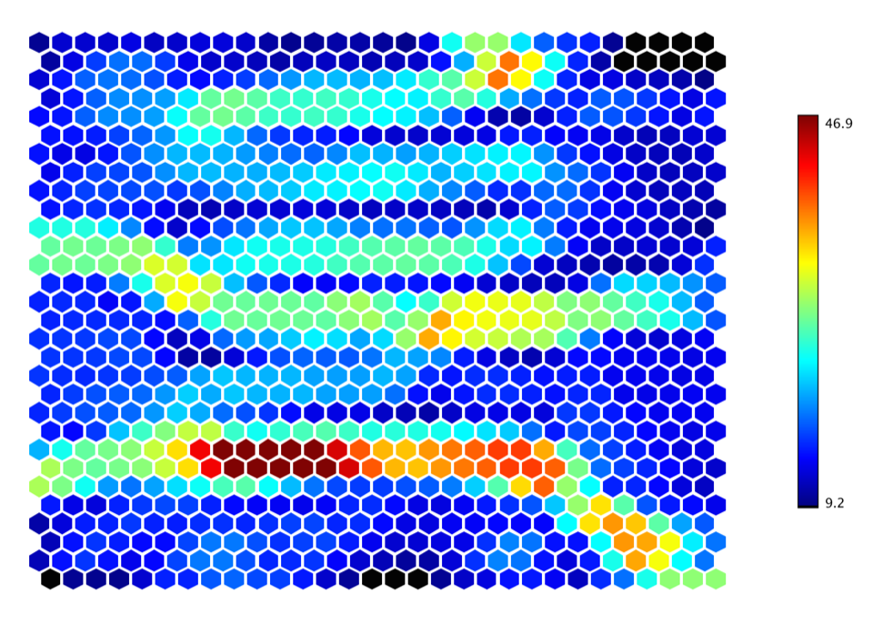
A common way to display SOMs is the heat map of U-matrix. The U-matrix value of a particular node is the minimum/maximum/average distance between the node and its closest neighbors. In a rectangular grid for instance, we might consider the closest 4 or 8 nodes. It is common to use the U-Matrix to visualize an SOM. The U-Matrix value of a particular node is the average distance between the node's weight vector and that of its closest neighbors. In a square grid, for instance, we might consider the closest 4 or 8 nodes (the Von Neumann and Moore neighborhoods, respectively), or six nodes in a hexagonal grid.
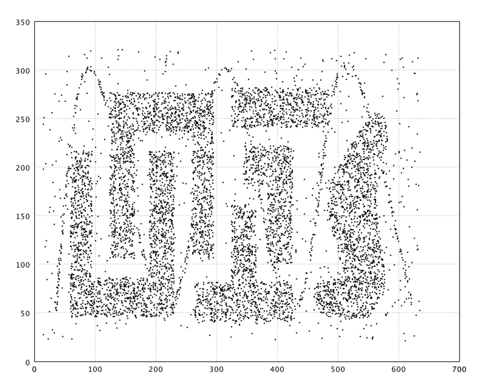
In what follows, we apply SOM to a complicated data from Chameleon
data set, as shown in the above. The SOM has 20 x 20
neurons.
    val x = read.csv("data/clustering/chameleon/t4.8k.txt", header=false, delimiter=" ").toArray

    val epochs = 20
    val lattice = SOM.lattice(20, 20, x)
    val som = new SOM(lattice,
                TimeFunction.constant(0.1),
                Neighborhood.Gaussian(1, x.length * epochs / 4))

    (1 to epochs).foreach { _ =>
        MathEx.permutate(x.length).foreach { i =>
            som.update(x(i));
        }
    }

    show(hexmap(som.umatrix, Palette.jet(256)))
    import smile.util.*;
    import smile.vq.*;
    var x = Read.csv("data/clustering/chameleon/t4.8k.txt", CSVFormat.DEFAULT.withDelimiter(' ')).toArray();

    var epochs = 20;
    var lattice = SOM.lattice(20, 20, x);
    var som = new SOM(lattice,
                TimeFunction.constant(0.1),
                Neighborhood.Gaussian(1, x.length * epochs / 4));

    for (int e = 0; e < epochs; e++) {
        for (int i : MathEx.permutate(x.length)) {
            som.update(x[i]);
        }
    }

    Hexmap.of(som.umatrix(), Palette.jet(256)).canvas().window();
The U-Matrix is visualized with a hexmap, where a dark red coloring between the neurons corresponds to a large distance and thus a gap between the codebook values in the input space. A dark blue coloring between the neurons signifies that the codebook vectors are close to each other in the input space. The blueish areas can be thought as clusters and reddish areas as cluster separators. This can be a helpful presentation when one tries to find clusters in the input data without having any a priori information about the clusters.
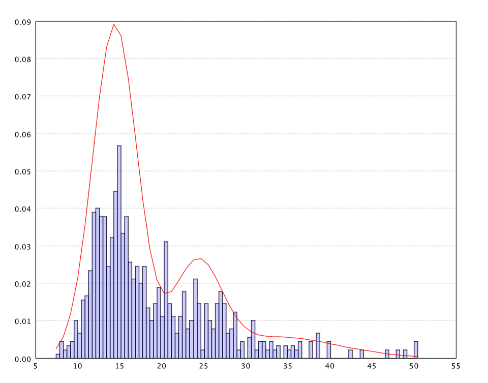
One may also fit a Gaussian mixture model on the U-Matrix values. Our implementation of EM algorithm to fix mixture models can automatically determine the number of components in the mixture. The distribution information can be used in other algorithms such as Guassian kernel smooth parameters, nearest neighbor range, etc.
    val dist = som.umatrix.flatten
    val canvas = hist(dist, 100, true)

    val mixture = GaussianMixture.fit(dist)

    val minDist = MathEx.min(dist)
    val w = (MathEx.max(dist) - minDist) / 50
    val pdf = (0 to 50).map { i =>
      val x = minDist + i * w
      val y = mixture.p(x) * w
      Array(x, y)
    }.toArray

    canvas.add(LinePlot.of(pdf, Color.RED))
    show(canvas)
    var dist = Arrays.stream(som.umatrix()).flatMapToDouble(r -> Arrays.stream(r)).toArray();
    var canvas = smile.plot.swing.Histogram.of(dist, 100, true).canvas();

    var mixture = GaussianMixture.fit(dist);

    var minDist = MathEx.min(dist);
    var w = (MathEx.max(dist) - minDist) / 50;
    var pdf = new double[51][2];
    for (int i = 0; i < pdf.length; i++) {
      pdf[i][0] = minDist + i * w;
      pdf[i][1] = mixture.p(pdf[i][0]) * w;
    }

    canvas.add(LinePlot.of(pdf, Color.RED));
    canvas.window();
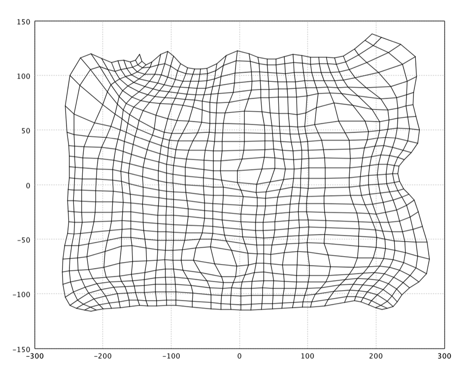
It is also common to visualize an SOM by mapping the neuron codebook vectors to a lower dimensional space (e.g. by Sammon's mapping).
    val codebook = som.neurons.flatten
    val codebook2d = sammon(pdist(codebook, false).toArray(), 2).coordinates

    val nodes = 20
    val neurons = (0 until nodes).map { i => codebook2d.slice(nodes*i, nodes*(i+1)) }.toArray
    show(grid(neurons))
    var codebook = Arrays.stream(som.neurons()).flatMap(r -> Arrays.stream(r)).toArray(double[][]::new);
    var codebook2d = SammonMapping.of(MathEx.pdist(codebook, false).toArray(), 2).coordinates;

    var nodes = 20;
    var neurons = new double[nodes][nodes][];
    for (int i = 0, k = 0; i < nodes; i++) {
        for (int j = 0; j < nodes; j++, k++) {
            neurons[i][j] = codebook2d[k];
        }
    }
    Grid.of(neurons).canvas().window();
Because this artificial data is 2-dimensional, it is not necessary to map the neurons in the SOM to a lower dimensional space. For demonstration, we still go through the whole process with a Sammon's mapping.
Neural Gas
The Neural Gas algorithm is inspired by the SOM for finding optimal data representations based on feature vectors. The algorithm was coined "Neural Gas" because of the dynamics of the feature vectors during the adaptation process, which distribute themselves like a gas within the data space. Although it is mainly applied where data compression or vector quantization is an issue, it is also used for cluster analysis as a robustly converging alternative to the k-means clustering.
Compared to SOM, neural gas has no topology of a fixed dimensionality (in fact, no topology at all). For each input signal during learning, the neural gas algorithm sorts the neurons of the network according to the distance of their reference vectors to the input signal. Based on this "rank order", neurons are adapted based on the adaptation strength that are decreased according to a fixed schedule.
The adaptation step of the Neural Gas can be interpreted as gradient descent on a cost function. By adapting not only the closest feature vector but all of them with a step size decreasing with increasing distance order, compared to k-means clustering, a much more robust convergence of the algorithm can be achieved.
val epochs = 20
val gas = new NeuralGas(NeuralGas.seed(400, x),
TimeFunction.exp(0.3, x.length * epochs / 2),
TimeFunction.exp(30, x.length * epochs / 8),
TimeFunction.constant(x.length * 2))
(1 to epochs).foreach { _ =>
MathEx.permutate(x.length).foreach { i =>
gas.update(x(i))
}
}
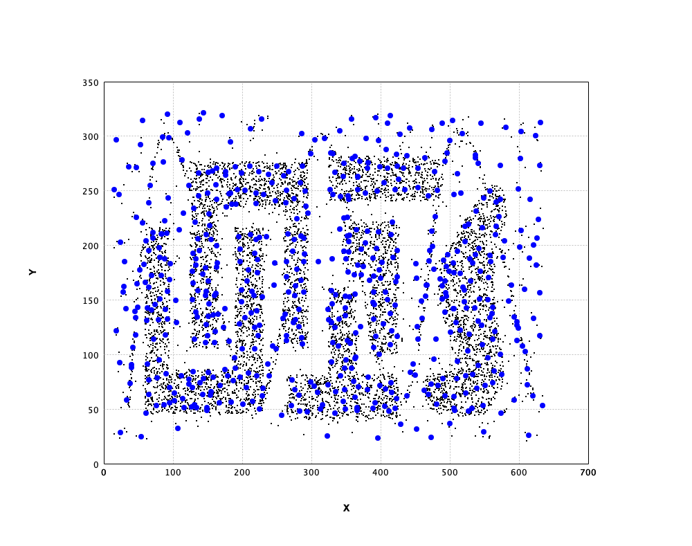
val canvas = plot(x, '.')
canvas.add(ScatterPlot.of(gas.neurons, '#', BLUE))
show(canvas)
    var epochs = 20;
    var gas = new NeuralGas(NeuralGas.seed(400, x),
                TimeFunction.exp(0.3, x.length * epochs / 2),
                TimeFunction.exp(30, x.length * epochs / 8),
                TimeFunction.constant(x.length * 2));

    for (int e = 0; e < epochs; e++) {
        for (int i : MathEx.permutate(x.length)) {
            gas.update(x[i]);
        }
    }

    var canvas = ScatterPlot.of(x, '.').canvas();
    canvas.add(ScatterPlot.of(gas.neurons(), '#', Color.BLUE));
    canvas.window();
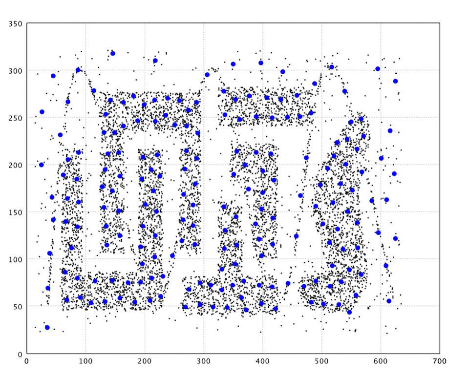
In the plot, we draw the neurons as big blue dots.
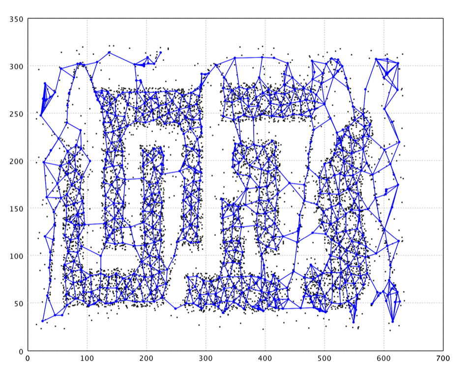
Growing Neural Gas
A prominent extension is the Growing Neural Gas (GNG). GNG can add and delete nodes during algorithm execution. The growth mechanism is based on growing cell structures and competitive Hebbian learning.
Compared to Neural Gas, GNG has the following distinctions:
- The system has the ability to add and delete nodes.
- Local Error measurements are noted at each step helping it to locally insert/delete nodes.
- Edges are connected between nodes, so a sufficiently old edges is deleted. Such edges are intended placeholders for localized data distribution.
- Such edges also help to locate distinct clusters (those clusters are not connected by edges).
    val gng = new GrowingNeuralGas(x(0).length)

    (1 to 10).foreach { _ =>
        MathEx.permutate(x.length).foreach { i =>
            gng.update(x(i))
        }
    }

    val neurons = gng.neurons
    val canvas = plot(x, '.')
    canvas.add(ScatterPlot.of(neurons.map(_.w).toArray, '@', BLUE))

    import scala.jdk.CollectionConverters._
    neurons.foreach { neuron =>
      neuron.edges.asScala.foreach { edge =>
        canvas.add(LinePlot.of(Array(neuron.w, edge.neighbor.w), BLUE))
      }
    }
    show(canvas)
    var gng = new GrowingNeuralGas(x[0].length);

    for (int e = 0; e < epochs; e++) {
        for (int i : MathEx.permutate(x.length)) {
            gng.update(x[i]);
        }
    }

    var neurons = gng.neurons();
    var canvas = ScatterPlot.of(x, '.').canvas();
    canvas.add(ScatterPlot.of(Arrays.stream(neurons).map(n -> n.w).toArray(double[][]::new), '@', Color.BLUE));

    Arrays.stream(neurons).forEach(neuron -> {
        neuron.edges.stream().forEach(edge -> {
            double[][] e = {neuron.w, edge.neighbor.w};
            canvas.add(LinePlot.of(e, Color.BLUE));
        });
    });
    canvas.window();
As shown in the plot, GNG nicely capture the structure of data. However, there are also neurons fitting noises and connecting clusters that should be separated. A further graph cut/clustering may help removing these neurons of noise.
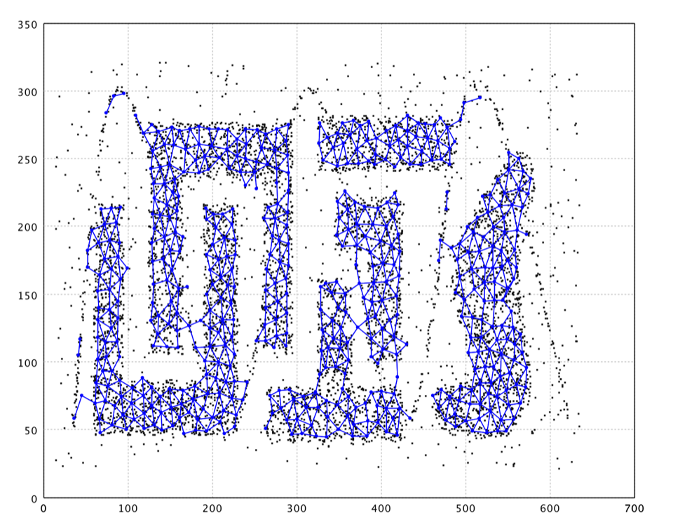
Neural Map
Neural Map is an efficient competitive learning algorithm inspired by growing neural gas and BIRCH. Like growing neural gas, Neural Map has the ability to add and delete neurons with competitive Hebbian learning. Edges exist between neurons close to each other. Such edges are intended placeholders for localized data distribution. Such edges also help to locate distinct clusters (those clusters are not connected by edges). Neural Map employs Locality-Sensitive Hashing to speed up the learning while BIRCH uses balanced CF trees.
    val cortex = new NeuralMap(x(0).length, 10, 0.01, 0.002, 50, 0.995)

    (1 to 5).foreach { _ =>
        MathEx.permutate(x.length).foreach { i =>
            cortex.update(x(i))
        }

        // Removes staled neurons and the edges beyond lifetime.
        cortex.clear(1E-7)
    }

    val neurons = cortex.neurons
    val canvas = plot(x, '.')
    canvas.add(ScatterPlot.of(neurons.map(_.w).toArray, '@', BLUE))

    import scala.jdk.CollectionConverters._
    neurons.foreach { neuron =>
      neuron.edges.asScala.foreach { edge =>
        canvas.add(LinePlot.of(Array(neuron.w, edge.neighbor.w), BLUE))
      }
    }
    show(canvas)
    var cortex = new NeuralMap(x[0].length, 10, 0.01, 0.002, 50, 0.995);

    for (int e = 0; e < 5; e++) {
        for (int i : MathEx.permutate(x.length)) {
            cortex.update(x[i]);
        }

        // Removes staled neurons and the edges beyond lifetime.
        cortex.clear(1E-7);
    }

    var neurons = cortex.neurons();
    var canvas = ScatterPlot.of(x, '.').canvas();
    canvas.add(ScatterPlot.of(Arrays.stream(neurons).map(n -> n.w).toArray(double[][]::new), '@', Color.BLUE));

    Arrays.stream(neurons).forEach(neuron -> {
        neuron.edges.stream().forEach(edge -> {
            double[][] e = {neuron.w, edge.neighbor.w};
            canvas.add(LinePlot.of(e, Color.BLUE));
        });
    });
    canvas.window();
Note that points in orange are outliers labeled by the algorithm.
BIRCH
BIRCH (Balanced Iterative Reducing and Clustering using Hierarchies) performs hierarchical clustering over particularly large datasets. An advantage of BIRCH is its ability to incrementally and dynamically cluster incoming, multidimensional metric data points in an attempt to produce the high quality clustering for a given set of resources (memory and time constraints).
BIRCH has several advantages. For example, each clustering decision is made without scanning all data points and currently existing clusters. It exploits the observation that data space is not usually uniformly occupied and not every data point is equally important. It makes full use of available memory to derive the finest possible sub-clusters while minimizing I/O costs. It is also an incremental method that does not require the whole data set in advance.
This implementation produces a clustering in three steps. First step builds a CF (clustering feature) tree by a single scan of database. The second step clusters the leaves of CF tree by hierarchical clustering. Then the user can use the learned model to cluster input data in the final step. In total, we scan the database twice.
A CF leaf will be treated as outlier if the number of its
points is less than the parameter minPts.
The branching factor parameter branch is the
maximum number of children nodes and the parameter radius
is the maximum radius of a sub-cluster.
    val birch = new BIRCH(x(0).length, 6, 3, 10)
    x.foreach { xi =>
        birch.update(xi)
    }

    val canvas = plot(x, '.')
    canvas.add(ScatterPlot.of(birch.centroids, '#', BLUE))
    show(canvas)
    var birch = new BIRCH(x[0].length, 6, 3, 10);
    for (double[] xi : x) {
        birch.update(xi);
    }

    var canvas = ScatterPlot.of(x, '.').canvas();
    canvas.add(ScatterPlot.of(birch.centroids(), '#', Color.BLUE));
    canvas.window();