Multi-Dimensional Scaling
Multidimensional scaling is a set of related statistical techniques often used in information visualization for exploring similarities or dissimilarities in data. An MDS algorithm starts with a matrix of item-item similarities, then assigns a location to each item in low-dimensional space. For sufficiently low dimension, the resulting locations may be displayed in a graph or 3D visualization.
The major types of MDS algorithms include:
- Classical multi-dimensional scaling
It takes an input matrix giving dissimilarities between pairs of items and outputs a coordinate matrix whose configuration minimizes a loss function called strain.
- Metric multi-dimensional scaling
A superset of classical MDS that generalizes the optimization procedure to a variety of loss functions and input matrices of known distances with weights and so on. A useful loss function in this context is called stress which is often minimized using a procedure called stress majorization.
- Non-metric multi-dimensional scaling
In contrast to metric MDS, non-metric MDS finds both a non-parametric monotonic relationship between the dissimilarities in the item-item matrix and the Euclidean distances between items, and the location of each item in the low-dimensional space. The relationship is typically found using isotonic regression.
- Generalized multi-dimensional scaling
An extension of metric multidimensional scaling, in which the target space is an arbitrary smooth non-Euclidean space. In case when the dissimilarities are distances on a surface and the target space is another surface, GMDS allows finding the minimum-distortion embedding of one surface into another.
Classical Multi-dimensional Scaling
Classical multidimensional scaling is also known as principal coordinates
analysis. Given a matrix A of dissimilarities (e.g. pairwise distances), MDS
finds a set of points in low dimensional space that well-approximates the
dissimilarities in A. We are not restricted to using a Euclidean
distance metric. However, when Euclidean distances are used, classical MDS is
equivalent to PCA.
def mds(proximity: Array[Array[Double]], k: Int, add: Boolean = false): MDS
    public class MDS {
        public static MDS fit(double[][] proximity, Options options);
    }
fun mds(proximity: Array<DoubleArray>, k: Int, add: Boolean = false): MDS
where proximity is the non-negative proximity matrix of dissimilarities.
The diagonal should be zero and all other elements should be positive and
symmetric. For pairwise distances matrix, it should be just the plain
distance, not squared.
The parameter k is the dimension of output space.
If the parameter add is true, the method estimates an appropriate constant to be added
to all the dissimilarities, apart from the self-dissimilarities, that
makes the learning matrix positive semi-definite. The other formulation of
the additive constant problem is as follows. If the proximity is
measured in an interval scale, where there is no natural origin, then there
is not a sympathy of the dissimilarities to the distances in the Euclidean
space used to represent the objects. In this case, we can estimate a constant c
such that proximity + c may be taken as ratio data, and also possibly
to minimize the dimensionality of the Euclidean space required for
representing the objects.
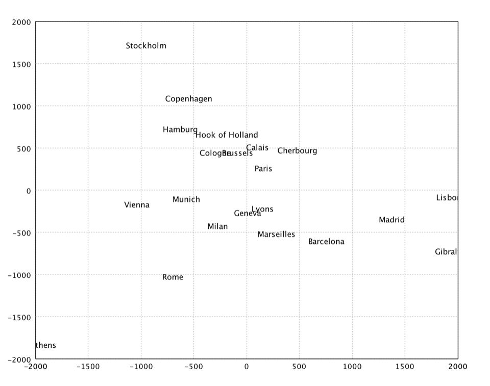
    val eurodist = read.csv("data/mds/eurodist.txt", delimiter = "\t", header = false)
    val dist = eurodist.drop(0).toArray()
    val citys = eurodist.stringVector(0).toArray()
    val x = mds(dist, 2).coordinates
    show(text(citys, x))
    var eurodist = Read.csv("data/mds/eurodist.txt", CSVFormat.DEFAULT.withDelimiter('\t'));
    var dist = eurodist.drop(0).toArray();
    var citys = eurodist.column(0).toStringArray();
    var x = MDS.fit(dist, new MDS.Options(2, true)).coordinates();
    var figure = TextPlot.of(citys, x).figure();
    show(figure);
    import smile.*;
    import smile.manifold.*;
    import smile.plot.swing.*;
    val eurodist = read.csv("data/mds/eurodist.txt", delimiter = '\t', header = false)
    val dist = eurodist.drop(0).toArray()
    val citys = eurodist.stringVector(0).toArray()
    val x = mds(dist, 2).coordinates
    TextPlot.of(citys, x).canvas().window()
In the above example, we apply MDS to a distance matrix of some European cities.
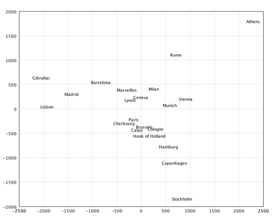
Kruskal's Nonmetric MDS
Kruskal's nonmetric MDS. In non-metric MDS, only the rank order of entries in the proximity matrix (not the actual dissimilarities) is assumed to contain the significant information. Hence, the distances of the final configuration should as far as possible be in the same rank order as the original data. Note that a perfect ordinal re-scaling of the data into distances is usually not possible. The relationship is typically found using isotonic regression.
def isomds(proximity: Array[Array[Double]], k: Int, tol: Double = 0.0001, maxIter: Int = 200): IsotonicMDS
    public class IsotonicMDS {
        public static IsotonicMDS fit(double[][] proximity, Options options);
    }
fun isomds(proximity: Array<DoubleArray>, k: Int, tol: Double = 0.0001, maxIter: Int = 200): IsotonicMDS
where tol is the tolerance for stopping iterations, and
maxIter is the maximum number of iterations.
    val x = isomds(dist, 2).coordinates
    show(text(citys, x))
    var x = IsotonicMDS.fit(dist).coordinates();
    var figure = TextPlot.of(citys, x).figure();
    show(figure);
    val x = isomds(dist, 2).coordinates
    TextPlot.of(citys, x).canvas().window()
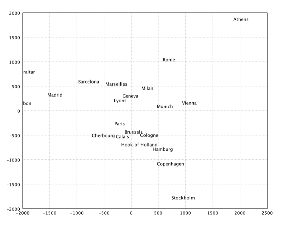
Sammon's Mapping
Sammon's mapping is an iterative technique for making interpoint distances in the low-dimensional projection as close as possible to the interpoint distances in the high-dimensional object. Two points close together in the high-dimensional space should appear close together in the projection, while two points far apart in the high dimensional space should appear far apart in the projection. The Sammon's mapping is a special case of metric least-square multidimensional scaling.
Ideally when we project from a high dimensional space to a low dimensional space the image would be geometrically congruent to the original figure. This is called an isometric projection. Unfortunately it is rarely possible to isometrically project objects down into lower dimensional spaces. Instead of trying to achieve equality between corresponding inter-point distances we can minimize the difference between corresponding inter-point distances. This is one goal of the Sammon's mapping algorithm. A second goal of the Sammon's mapping algorithm is to preserve the topology as good as possible by giving greater emphasize to smaller interpoint distances. The Sammon's mapping algorithm has the advantage that whenever it is possible to isometrically project an object into a lower dimensional space it will be isometrically projected into the lower dimensional space. But whenever an object cannot be projected down isometrically the Sammon's mapping projects it down to reduce the distortion in interpoint distances and to limit the change in the topology of the object.
The projection cannot be solved in a closed form and may be found by an iterative algorithm such as gradient descent suggested by Sammon. Kohonen also provides a heuristic that is simple and works reasonably well.
def sammon(proximity: Array[Array[Double]], k: Int, lambda: Double = 0.2, tol: Double = 0.0001, maxIter: Int = 100): SammonMapping
    public class SammonMapping {
        public static SammonMapping fit(double[][] proximity, Options options);
    }
fun sammon(proximity: Array<DoubleArray>, k: Int, lambda: Double = 0.2, tol: Double = 0.0001, maxIter: Int = 100): SammonMapping
where lambda is the initial value of the step size constant in diagonal Newton method.
    val x = sammon(dist, 2).coordinates
    show(text(citys, x))
    var x = SammonMapping.fit(dist).coordinates();
    var figure = TextPlot.of(citys, x).figure();
    show(figure);
    val x = sammon(dist, 2).coordinates
    TextPlot.of(citys, x).canvas().window()