Manifold Learning
Manifold learning finds a low-dimensional basis for describing high-dimensional data. Manifold learning is a popular approach to nonlinear dimensionality reduction. Algorithms for this task are based on the idea that the dimensionality of many data sets is only artificially high; though each data point consists of perhaps thousands of features, it may be described as a function of only a few underlying parameters. That is, the data points are actually samples from a low-dimensional manifold that is embedded in a high-dimensional space. Manifold learning algorithms attempt to uncover these parameters in order to find a low-dimensional representation of the data.
Some prominent approaches are locally linear embedding (LLE), Hessian LLE, Laplacian eigenmaps, and LTSA. These techniques construct a low-dimensional data representation using a cost function that retains local properties of the data, and can be viewed as defining a graph-based kernel for Kernel PCA. More recently, techniques have been proposed that, instead of defining a fixed kernel, try to learn the kernel using semidefinite programming. The most prominent example of such a technique is maximum variance unfolding (MVU). The central idea of MVU is to exactly preserve all pairwise distances between nearest neighbors (in the inner product space), while maximizing the distances between points that are not nearest neighbors.
An alternative approach to neighborhood preservation is through the minimization of a cost function that measures differences between distances in the input and output spaces. Important examples of such techniques include classical multidimensional scaling (which is identical to PCA), Isomap (which uses geodesic distances in the data space), diffusion maps (which uses diffusion distances in the data space), t-SNE (which minimizes the divergence between distributions over pairs of points), and curvilinear component analysis.
Isomap
Isometric feature mapping (isomap) is a widely used low-dimensional embedding methods, where geodesic distances on a weighted graph are incorporated with the classical multidimensional scaling. Isomap is used for computing a quasi-isometric, low-dimensional embedding of a set of high-dimensional data points. Isomap is highly efficient and generally applicable to a broad range of data sources and dimensionalities.
To be specific, the classical MDS performs low-dimensional embedding based
on the pairwise distance between data points, which is generally measured
using straight-line Euclidean distance. Isomap is distinguished by
its use of the geodesic distance induced by a neighborhood graph
embedded in the classical scaling. This is done to incorporate manifold
structure in the resulting embedding. Isomap defines the geodesic distance
to be the sum of edge weights along the shortest path between two nodes.
The top n eigenvectors of the geodesic distance matrix, represent the
coordinates in the new n-dimensional Euclidean space.
def isomap(data: Array[Array[Double]], k: Int, d: Int = 2, CIsomap: Boolean = true): Array[Array[Double]]
    public class IsoMap {
        public static double[][] fit(double[][] data, Options options);
        public static double[][] fit(NearestNeighborGraph nng, Options options);
    }
fun isomap(data: Array<DoubleArray>, k: Int, d: Int = 2, CIsomap: Boolean = true): Array<DoubleArray>
The connectivity of each data point in the neighborhood graph is defined
as its nearest k Euclidean neighbors in the high-dimensional space. This
step is vulnerable to "short-circuit errors" if k is too large with
respect to the manifold structure or if noise in the data moves the
points slightly off the manifold. Even a single short-circuit error
can alter many entries in the geodesic distance matrix, which in turn
can lead to a drastically different (and incorrect) low-dimensional
embedding. Conversely, if k is too small, the neighborhood graph may
become too sparse to approximate geodesic paths accurately.
When the optional parameter CIsomap is true, the method
performs C-Isomap that involves magnifying the regions
of high density and shrink the regions of low density of data points
in the manifold. Edge weights that are maximized in Multi-Dimensional
Scaling(MDS) are modified, with everything else remaining unaffected.
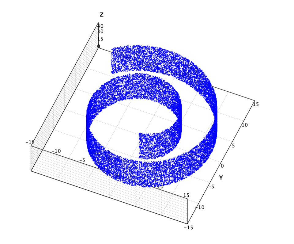
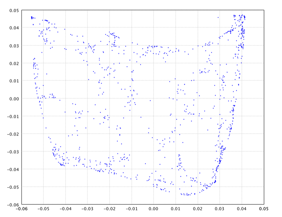
In the below example, we apply Isomap to the famous swiss roll data as shown above. This data set was created to test out various dimensionality reduction algorithms. The idea was to create several points in 2d, and then map them to 3d with some smooth function, and then to see what the algorithm would find when it mapped the points back to 2d. The data contains 20,000 samples. Because it is computational intensive to calculate the shortest path for all samples, the example uses only the first 2,000 samples.
    val swissroll = read.csv("data/manifold/swissroll.txt", header=false, delimiter="\t").toArray()
    show(plot(swissroll, '.', BLUE))

    val data = swissroll.slice(0, 2000)
    val map = isomap(data, 7)
    show(plot(map, '.', BLUE))
    var swissroll = Read.csv("data/manifold/swissroll.txt", CSVFormat.DEFAULT.withDelimiter('\t')).toArray();
    ScatterPlot.of(swissroll, '.', Color.BLUE).canvas().window();

    var data = Arrays.copyOf(swissroll, 2000);
    var nng = NearestNeighborGraph.descent(data, MathEx::distance, 7).largest(false);
    var map = IsoMap.fit(nng, 2, false);

    var graph = nng.graph(false);
    var edges = IntStream.range(0, data.length)
            .mapToObj(graph::getEdges)
            .flatMap(List::stream)
            .map(edge -> new int[]{edge.u(), edge.v()})
            .toArray(int[][]::new);
    var figure = Wireframe.of(map, edges).figure();
    show(figure);
    import java.awt.Color;
    import smile.*;
    import smile.manifold.*;
    import smile.plot.swing.*;

    val swissroll = read.csv("data/manifold/swissroll.txt", header=false, delimiter='\t').toArray();
    ScatterPlot.of(swissroll, '.', Color.BLUE).canvas().window();

    val data = swissroll.slice(0..2000).toTypedArray()
    val map = isomap(data, 7);
    ScatterPlot.of(map, '.', Color.BLUE).canvas().window();
In this example, we use k = 7 for neighborhood graph. In the mapped
2d space, we also plot the connections between neighbor neighbors.
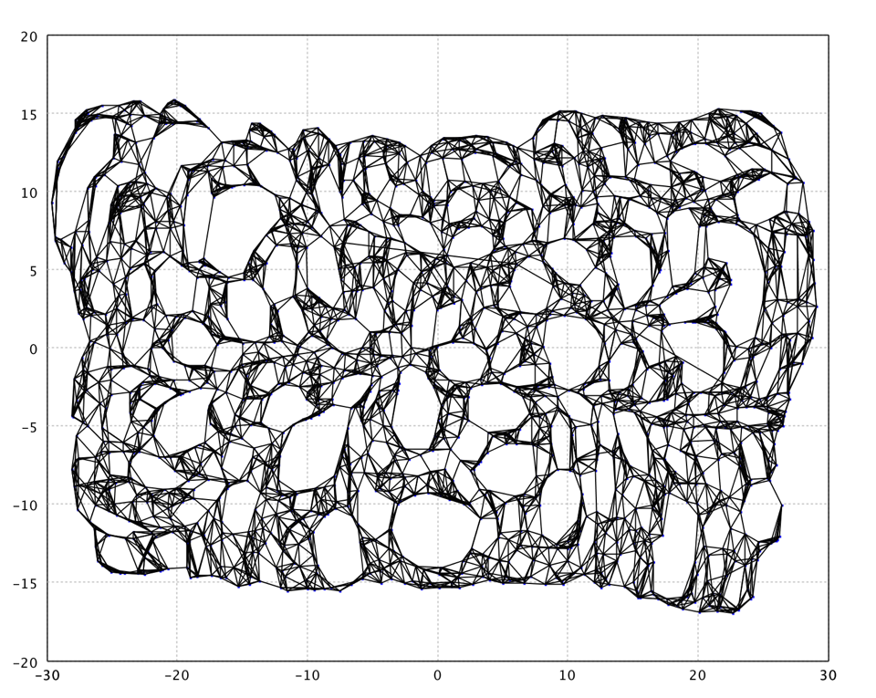
Note that Isomap produces strange holes like in a slice of Swiss cheese :). This issue can be solved by adding to Isomap a vector quantization step.
LLE
Locally Linear Embedding (LLE) has several advantages over Isomap, including faster optimization when implemented to take advantage of sparse matrix algorithms, and better results with many problems. LLE also begins by finding a set of the nearest neighbors of each point. It then computes a set of weights for each point that best describe the point as a linear combination of its neighbors. Finally, it uses an eigenvector-based optimization technique to find the low-dimensional embedding of points, such that each point is still described with the same linear combination of its neighbors. LLE tends to handle non-uniform sample densities poorly because there is no fixed unit to prevent the weights from drifting as various regions differ in sample densities.
def lle(data: Array[Array[Double]], k: Int, d: Int = 2): Array[Array[Double]]
    public class LLE {
        public static double[][] fit(double[][] data, Options options);
        public static double[][] fit(double[][] data, NearestNeighborGraph nng, Options options);
    }
fun lle(data: Array<DoubleArray>, k: Int, d: Int = 2): Array<DoubleArray>
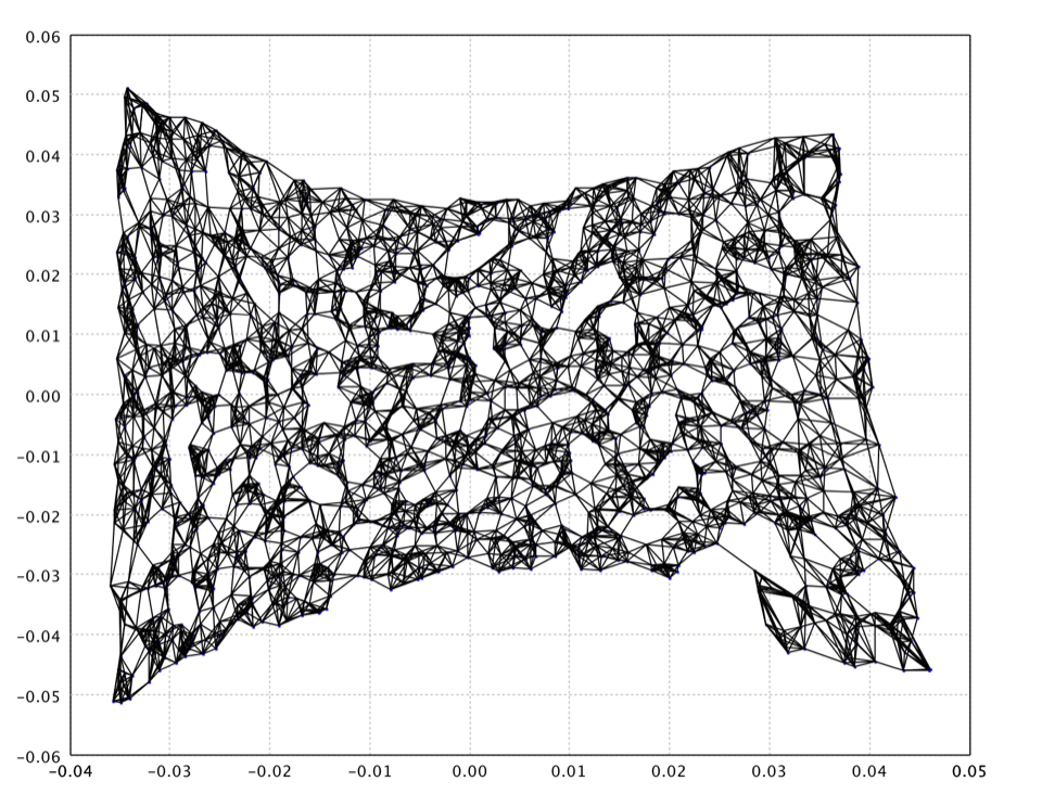
The LLE using 8 neighbors on the swiss roll data is as follows.
val map = lle(data, 2)
var map = LLE.fit(data, nng, 2);
val map = lle(data, 8)
Laplacian Eigenmap
Using the notion of the Laplacian of the nearest neighbor adjacency graph, Laplacian Eigenmap computes a low dimensional representation of the dataset that optimally preserves local neighborhood information in a certain sense. The representation map generated by the algorithm may be viewed as a discrete approximation to a continuous map that naturally arises from the geometry of the manifold.
def laplacian(data: Array[Array[Double]], k: Int, d: Int = 2, t: Double = -1): Array[Array[Double]]
    public class LaplacianEigenmap {
        public static double[][] fit(double[][] data, Options options);
        public static double[][] fit(NearestNeighborGraph nng, Options options);
    }
fun laplacian(data: Array<DoubleArray>, k: Int, d: Int = 2, t: Double = -1): Array<DoubleArray>
where t is the smooth/width parameter of heat kernel
e-||x-y||2/t.
Non-positive t means discrete weights.
The locality preserving character of the Laplacian Eigenmap algorithm makes it relatively insensitive to outliers and noise. It is also not prone to "short-circuiting" as only the local distances are used.
The Laplacian Eigenmap on the swiss roll data is as follows.
val map = laplacian(swissroll.slice(0, 1000), 10, 2, 25.0)
var map = LaplacianEigenmap.fit(nng, 2, 25.0);
val map = laplacian(swissroll.slice(0..1000).toTypedArray(), 10, 2, 25.0)
t-SNE
The t-distributed stochastic neighbor embedding (t-SNE) is a nonlinear dimensionality reduction technique that is particularly well suited for embedding high-dimensional data into a space of two or three dimensions, which can then be visualized in a scatter plot. Specifically, it models each high-dimensional object by a two- or three-dimensional point in such a way that similar objects are modeled by nearby points and dissimilar objects are modeled by distant points.
    def tsne(X: Array[Array[Double]],
             d: Int = 2,
             perplexity: Double = 20.0,
             eta: Double = 200.0,
             iterations: Int = 1000): TSNE
    public class TSNE {
        public static TSNE fit(double[][] X, Options options);
    }
    fun tsne(X: Array<DoubleArray>,
             d: Int = 2,
             perplexity: Double = 20.0,
             eta: Double = 200.0,
             iterations: Int = 1000): TSNE
where X is input data, perplexity is the perplexity
of the conditional distribution, eta the learning rate, and iterations is
the number of iterations. If X is a square matrix, it is assumed
to be the distance/dissimilarity matrix.
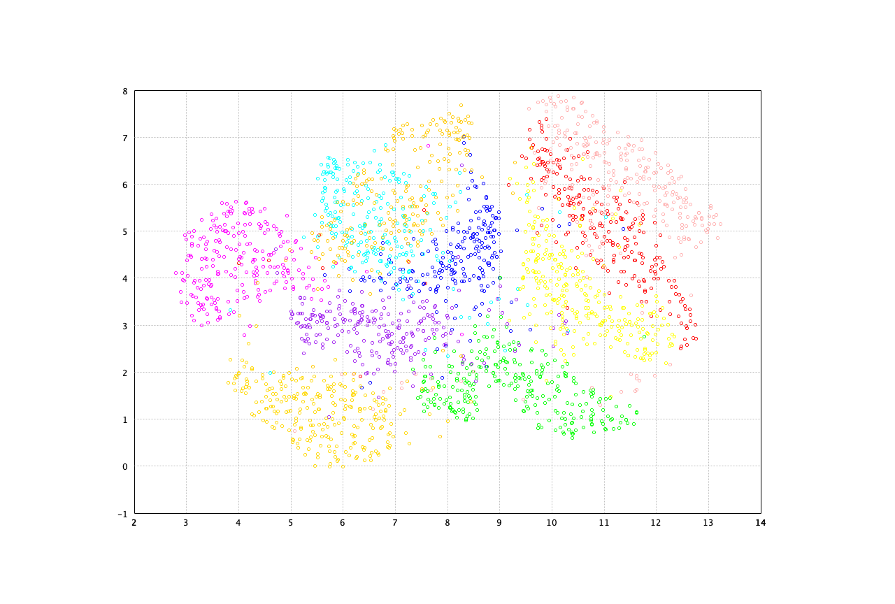
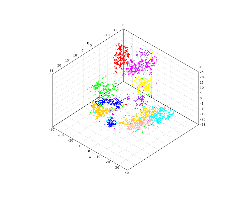
The t-SNE on the MNIST data is as follows. Note that the input data is preprocessed using PCA to reduce the dimensionality to 50 before t-SNE is performed.
    val mnist = read.csv("data/mnist/mnist2500_X.txt", header=false, delimiter=" ")
    val label = read.csv("data/mnist/mnist2500_labels.txt", header=false, delimiter=" ").column(0).toIntArray()
    val pc = pca(mnist).getProjection(50)
    val x50 = pc(mnist).toArray()
    val sne = tsne(x50, 3, 20, 200, 1000)
    show(plot(sne.coordinates, label, 'o'))
    var format = CSVFormat.DEFAULT.withDelimiter(' ');
    var mnist = Read.csv("data/mnist/mnist2500_X.txt", format).toArray();
    var label = Read.csv("data/mnist/mnist2500_labels.txt", format).column(0).toIntArray();

    var pca = PCA.fit(mnist).getProjection(50);
    var X = pca.apply(mnist);
    var tsne = TSNE.fit(X, new TSNE.Options(2, 20, 200, 12, 550));

    var figure = ScatterPlot.of(tsne.coordinates(), label, '@').figure();
    figure.setTitle("t-SNE of MNIST");
    show(figure);
    import smile.feature.extraction.*;
    val mnist = read.csv("data/mnist/mnist2500_X.txt", header=false, delimiter=' ').toArray();
    val label = read.csv("data/mnist/mnist2500_labels.txt", header=false, delimiter=' ').column(0).toIntArray();
    val pc = pca(mnist).getProjection(50);
    val x50 = pc.apply(mnist);
    val sne = tsne(x50, 3, 20.0, 200.0, 1000);

    val canvas = ScatterPlot.of(sne.coordinates, label, '@').canvas();
    canvas.setTitle("t-SNE of MNIST");
    canvas.window();
UMAP
Uniform Manifold Approximation and Projection can be used for visualization similarly to t-SNE, but also for general non-linear dimension reduction. The algorithm is founded on three assumptions about the data:
- The data is uniformly distributed on a Riemannian manifold;
- The Riemannian metric is locally constant (or can be approximated as such);
- The manifold is locally connected.
From these assumptions it is possible to model the manifold with a fuzzy topological structure. The embedding is found by searching for a low dimensional projection of the data that has the closest possible equivalent fuzzy topological structure.
    def umap(data: Array[Array[Double]],
             k: Int = 15,
             d: Int = 2,
             epochs: Int = 0,
             learningRate: Double = 1.0,
             minDist: Double = 0.1,
             spread: Double = 1.0,
             negativeSamples: Int = 5,
             repulsionStrength: Double = 1.0,
             localConnectivity: Double = 1.0): Array[Array[Double]]
    public class UAMP {
        public double[][] fit(double[][] data, Options options);

        public double[][] fit(T[] data, Metric>T< distance, Options options);

        public double[][] fit(T[] data, NearestNeighborGraph nng, Options options);
    }
    fun umap(data: Array<DoubleArray>,
             k: Int = 15,
             d: Int = 2,
             epochs: Int = 0,
             learningRate: Double = 1.0,
             minDist: Double = 0.1,
             spread: Double = 1.0,
             negativeSamples: Int = 5,
             repulsionStrength: Double = 1.0,
             localConnectivity: Double = 1.0): Array<DoubleArray>
where data is the input data, k is of
k-nearest neighbors. Larger values result in more global views
of the manifold, while smaller values result in more local data
being preserved. d is the target embedding dimensions.
iterations is the number of iterations to optimize the
low-dimensional representation. Larger values result in more
accurate embedding. Muse be greater than 10. Choose wise value
based on the size of the input data, e.g, 200 for large
data (1000+ samples), 500 for small.
learningRate is the initial learning rate for the
embedding optimization.
minDist is the desired separation between close points
in the embedding space. Smaller values will result in a more
clustered/clumped embedding where nearby points on the manifold are
drawn closer together, while larger values will result on a more even
disperse of points. The value should be set no-greater than
and relative to the spread value, which determines the scale
at which embedded points will be spread out.
spread is the effective scale of embedded points.
In combination with minDist, this determines how
clustered/clumped the embedded points are.
negativeSamples is the number of negative samples to
select per positive sample in the optimization process. Increasing
this value will result in greater repulsive force being applied,
greater optimization cost, but slightly more accuracy.
repulsionStrengthplied to negative samples in low
dimensional embedding optimization. Values higher than one will result
in greater weight being given to negative samples.
UMAP on the MNIST data is as follows.
    val map = umap(mnist.toArray())
    show(plot(map, label, 'o'))
    var map = UMAP.fit(mnist, 15);
    ScatterPlot.of(map, label, '@').canvas().window();
    val map = umap(mnist);
    ScatterPlot.of(map, label, '@').canvas().window();