Feature Engineering
We have gone through the classification and regression algorithms. In the examples, we assume that the data is ready and features are carefully prepared, which many machine learning practitioners take as granted. However, it is not general case in practice. The practitioners should pay a lot of attentions on feature generation, selection, and dimension reduction, which often have bigger impacts on the final results than the choice of particular learning algorithm.
Understanding the problem (and the business) is the most important thing to prepare the features. Besides the attributes supplied with the training instances, researchers should modify or enhance the representation of data objects in search of new features that describe the objects better.
The accuracy of the inferred function depends strongly on how the input object is represented. Typically, the input object is transformed into a feature vector, which contains a number of features that are descriptive of the object. The number of features should not be too large because of the curse of dimensionality; but should contain enough information to accurately predict the output. Beyond feature vectors, a few algorithms such as support vector machines can process complex data object such as sequences, trees, and even graphs with properly engineered kernels.
If each of the features makes an independent contribution to the output, then algorithms based on linear functions (e.g., linear regression, logistic regression, linear support vector machines, naive Bayes) generally perform well. However, if there are complex interactions among features, then algorithms such as nonlinear support vector machines, decision trees and neural networks work better. Linear methods can also be applied, but engineers must manually specify the interactions when using them.
If the input features contain redundant information (e.g., highly correlated features), some learning algorithms (e.g., linear regression, logistic regression, and distance based methods) will perform poorly because of numerical instabilities. These problems can often be solved by imposing some form of regularization.
Preprocessing
Many machine learning methods such as Neural Networks and SVM with Gaussian
kernel also require the features properly scaled/standardized. For example,
each variable is scaled into interval [0, 1] or to have mean 0 and standard
deviation 1. Methods that employ a distance function are particularly sensitive
to this. In the package smile.feature, we provide several classes
to preprocess the features. These classes generally learn the transform from
a training data and can be applied to new feature vectors.
The class Scaler scales all numeric variables into the range [0, 1].
If the dataset has outliers, normalization will certainly scale
the "normal" data to a very small interval. In this case, the
Winsorization procedure should be applied: values greater than the
specified upper limit are replaced with the upper limit, and those
below the lower limit are replace with the lower limit. Often, the
specified range is indicate in terms of percentiles of the original
distribution (like the 5th and 95th percentile). The class WinsorScaler
implements this algorithm. In additional, the class MaxAbsScaler
scales each feature by its maximum absolute value so that the maximal absolute value
of each feature in the training set will be 1.0. It does not shift/center
the data, and thus does not destroy any sparsity.
    import smile.base.mlp.Layer;
    var pendigits = Read.csv("data/classification/pendigits.txt", CSVFormat.DEFAULT.withDelimiter('\t'));
    var df = pendigits.drop(16);
    var y = pendigits.column(16).toIntArray();
    var scaler = WinsorScaler.fit(df, 0.01, 0.99);
    var x = scaler.apply(df).toArray();

    CrossValidation.classification(10, x, y, (x, y) -> {
        var model = new smile.classification.MLP(Layer.input(16),
                    Layer.sigmoid(50),
                    Layer.mle(10, OutputFunction.SIGMOID)
            );

        for (int epoch = 0; epoch < 10; epoch++) {
            for (int i : MathEx.permutate(x.length)) {
                model.update(x[i], y[i]);
            }
        }

        return model;
    });
The class Standardizer transforms numeric feature to 0 mean and unit variance.
Standardization makes an assumption that the data follows
a Gaussian distribution and are also not robust when outliers present.
A robust alternative is to subtract the median and divide by the IQR, which
is implemented RobustStandardizer.
    var zip = Read.csv("data/usps/zip.train", CSVFormat.DEFAULT.withDelimiter(' '));
    var df = zip.drop(0);
    var y = zip.column(0).toIntArray();

    var scaler = Standardizer.fit(df);
    var x = scaler.apply(df).toArray();

    var model = new smile.classification.MLP(Layer.input(256),
                Layer.sigmoid(768),
                Layer.sigmoid(192),
                Layer.sigmoid(30),
                Layer.mle(10, OutputFunction.SIGMOID)
        );

    model.setLearningRate(TimeFunction.constant(0.1));
    model.setMomentum(TimeFunction.constant(0.0));

    for (int epoch = 0; epoch < 10; epoch++) {
        for (int i : MathEx.permutate(x.length)) {
            model.update(x[i], y[i]);
        }
    }
The class Normalizer transform samples to unit norm. This class
is stateless and thus doesn't need to learn transformation parameters from data.
Each sample (i.e. each row of the data matrix) with at least one non-zero
component is rescaled independently of other samples so that its norm
(L1 or L2) equals one. Scaling inputs to unit norms is a common operation for text
classification or clustering for instance.
The class smile.math.MathEx also provides several functions for
similar purpose, such as standardize(), normalize(),
and scale() that apply to a matrix.
Although some method such as decision trees can handle nominal variable directly,
other methods generally require nominal variables converted to multiple binary
dummy variables to indicate the presence or absence of a characteristic.
The class OneHotEncoder encode categorical integer features
using the one-of-K scheme.
There are other feature generation classes in the package. For example,
DateFeature generates the attributes of Date object.
Bag is a generic implementation of bag of words features, which
may be applied to generic objects other than String.
Hughes Effect
In practice, we often start with generating a lot of features with the hope that
more relevant information will improve the accuracy. However, it is not always
good to include a large number of features in the learning system.
It is well known that the optimal rate of convergence to fit the
m-th derivate of θ (θ is a p-times differentiable regression
function, especially nonparametric ones) to the data is at best proportional
to n-(p-m)/(2p+d), where n is the number
of data points, and d is the dimensionality of the data.
In a nutshell, the rate of convergence will be exponentially slower
when we increase the dimensionality of our inputs. In other words,
with a fixed number of training samples, the predictive power reduces
as the dimensionality increases, known as the Hughes effect.
Therefore, feature selection that identifies the relevant features and discards the irrelevant ones and dimension reduction that maps the input data into a lower dimensional space are generally required prior to running the supervised learning algorithm.
Feature Selection
Feature selection is the technique of selecting a subset of relevant features for building robust learning models. By removing most irrelevant and redundant features from the data, feature selection helps improve the performance of learning models by alleviating the effect of the curse of dimensionality, enhancing generalization capability, speeding up learning process, etc. More importantly, feature selection also helps researchers to acquire better understanding about the data.
Feature selection algorithms typically fall into two categories: feature ranking and subset selection. Feature ranking methods rank the features by a metric and eliminate all features that do not achieve an adequate score. Subset selection searches the set of possible features for the optimal subset. Clearly, an exhaustive search of optimal subset is impractical if large numbers of features are available. Commonly, heuristic methods such as genetic algorithms are employed for subset selection.
Signal Noise Ratio
The signal-to-noise (S2N) metric ratio is a univariate feature ranking metric, which can be used as a feature selection criterion for binary classification problems. S2N is defined as
|μ1 - μ2| / (σ1 + σ2)
where μ1 and μ2 are the mean value of the variable in classes 1 and 2, respectively, and σ1 and σ2 are the standard deviations of the variable in classes 1 and 2, respectively. Clearly, features with larger S2N ratios are better for classification.
The output is the S2N ratios for each variable.
Sum Squares Ratio
The ratio of between-groups to within-groups sum of squares is a univariate feature ranking metric, which can be used as a feature selection criterion for multi-class classification problems. For each variable j, this ratio is
BSS(j) / WSS(j) = ΣI(yi = k)(xkj - x·j)2 / ΣI(yi = k)(xij - xkj)2
where x·j denotes the average of variable j across all samples, xkj denotes the average of variable j across samples belonging to class k, and xij is the value of variable j of sample i. Clearly, features with larger sum squares ratios are better for classification.
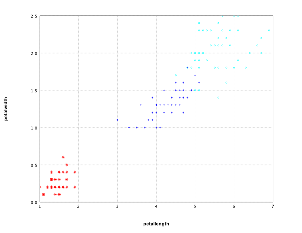
Applying it to Iris data, we can find that the last two variables have much higher sum squares ratios (about 16 and 13 in contrast to 1.6 and 0.6 of the first two variables).
    var iris = Read.arff("data/weka/iris.arff");
    SumSquaresRatio.fit(iris, "class");

    var df = iris.select("petallength", "petalwidth", "class");
    var canvas = ScatterPlot.of(df, "petallength", "petalwidth", "class", '*').canvas();
    canvas.setAxisLabels(iris.names()[2], iris.names()[3]);
    canvas.window();
The scatter plot of the last two variables shows clearly that they capture the difference among classes.
Ensemble Learning Based Feature Selection
Ensemble learning methods (e.g. random forest, gradient boosted trees, and AdaBoost) can give the estimates of what variables are important in the classification. Every time a split of a node is made on variable the (GINI, information gain, etc.) impurity criterion for the two descendent nodes is less than the parent node. Adding up the decreases for each individual variable over all trees in the forest gives a fast variable importance that is often very consistent with the permutation importance measure.
For these algorithms, there is a method importance returning
the scores for feature selection (higher is better).
    val iris = read.arff("data/weka/iris.arff")
    val model = smile.classification.randomForest("class" ~ ".", iris)
    println(iris.names.slice(0, 4).zip(model.importance).mkString("\n"))
    var model = smile.classification.RandomForest.fit(Formula.lhs("class"), iris);
    for (int i = 0; i < 4; i++) {
        System.out.format("%s\t%.2f\n", iris.names()[i], model.importance()[i]);
    }
For Iris data, random forest also gives much higher importance scores for the last two variables.
For data including categorical variables with different number of levels, random forests are biased in favor of those attributes with more levels. Therefore, the variable importance scores from random forest are not reliable for this type of data.
TreeSHAP
SHAP (SHapley Additive exPlanations) is a game theoretic approach to explain the output of any machine learning model. It connects optimal credit allocation with local explanations using the classic Shapley values from game theory. In game theory, the Shapley value is the average expected marginal contribution of one player after all possible combinations have been considered.
SHAP leverages local methods designed to explain a prediction f(x)
based on a single input x. The local methods are defined
as any interpretable approximation of the original model. In particular,
SHAP employs additive feature attribution methods.
SHAP values attribute to each feature the change in the expected
model prediction when conditioning on that feature. They explain
how to get from the base value E[f(z)] that would be
predicted if we did not know any features to the current output
f(x).
Tree SHAP is a fast and exact method to estimate SHAP values for tree models and ensembles of trees, under several different possible assumptions about feature dependence.
smile> val housing = read.arff("data/weka/regression/housing.arff")
[main] INFO smile.io.Arff - Read ARFF relation housing
housing: DataFrame = [CRIM: float, ZN: float, INDUS: float, CHAS: byte nominal[0, 1], NOX: float, RM: float, AGE: float, DIS: float, RAD: float, TAX: float, PTRATIO: float, B: float, LSTAT: float, class: float]
+------+----+-----+----+-----+-----+----+------+---+---+-------+------+-----+-----+
|  CRIM|  ZN|INDUS|CHAS|  NOX|   RM| AGE|   DIS|RAD|TAX|PTRATIO|     B|LSTAT|class|
+------+----+-----+----+-----+-----+----+------+---+---+-------+------+-----+-----+
|0.0063|  18| 2.31|   0|0.538|6.575|65.2|  4.09|  1|296|   15.3| 396.9| 4.98|   24|
|0.0273|   0| 7.07|   0|0.469|6.421|78.9|4.9671|  2|242|   17.8| 396.9| 9.14| 21.6|
|0.0273|   0| 7.07|   0|0.469|7.185|61.1|4.9671|  2|242|   17.8|392.83| 4.03| 34.7|
|0.0324|   0| 2.18|   0|0.458|6.998|45.8|6.0622|  3|222|   18.7|394.63| 2.94| 33.4|
| 0.069|   0| 2.18|   0|0.458|7.147|54.2|6.0622|  3|222|   18.7| 396.9| 5.33| 36.2|
|0.0299|   0| 2.18|   0|0.458| 6.43|58.7|6.0622|  3|222|   18.7|394.12| 5.21| 28.7|
|0.0883|12.5| 7.87|   0|0.524|6.012|66.6|5.5605|  5|311|   15.2| 395.6|12.43| 22.9|
|0.1445|12.5| 7.87|   0|0.524|6.172|96.1|5.9505|  5|311|   15.2| 396.9|19.15| 27.1|
|0.2112|12.5| 7.87|   0|0.524|5.631| 100|6.0821|  5|311|   15.2|386.63|29.93| 16.5|
|  0.17|12.5| 7.87|   0|0.524|6.004|85.9|6.5921|  5|311|   15.2|386.71| 17.1| 18.9|
+------+----+-----+----+-----+-----+----+------+---+---+-------+------+-----+-----+
496 more rows...

smile> val model = smile.regression.randomForest("class" ~ ".", housing)
[main] INFO smile.util.package$ - Random Forest runtime: 0:00:00.495102
model: regression.RandomForest = smile.regression.RandomForest@52d63b7e

smile> println(housing.names.slice(0, 13).zip(model.importance).sortBy(_._2).map(t => "%-15s %12.4f".format(t._1, t._2)).mkString("\n"))
CHAS              87390.1358
ZN               139917.2980
RAD              142194.2660
B                290043.4817
AGE              442444.4313
TAX              466142.1004
DIS             1006704.7537
CRIM            1067521.2371
INDUS           1255337.3748
NOX             1265518.8700
PTRATIO         1402827.4712
LSTAT           6001941.3822
RM              6182463.1457

smile> println(housing.names.slice(0, 13).zip(model.shap(housing.stream.parallel)).sortBy(_._2).map(t => "%-15s %12.4f".format(t._1, t._2)).mkString("\n"))
CHAS                  0.0483
ZN                    0.0514
RAD                   0.0601
B                     0.1647
AGE                   0.2303
TAX                   0.2530
DIS                   0.3403
CRIM                  0.5217
INDUS                 0.5734
NOX                   0.6423
PTRATIO               0.7819
RM                    2.3272
LSTAT                 2.6838
smile> import smile.io.*

smile> import smile.data.formula.*

smile> import smile.regression.*

smile> var housing = Read.arff("data/weka/regression/housing.arff")
[main] INFO smile.io.Arff - Read ARFF relation housing
housing ==> [CRIM: float, ZN: float, INDUS: float, CHAS: byte ... -+-----+
496 more rows...

smile> var model = smile.regression.RandomForest.fit(Formula.lhs("class"), housing)
model ==> smile.regression.RandomForest@6b419da

smile> var importance = model.importance()
importance ==> double[13] { 1055236.1223483568, 140436.296249959 ... 12613, 5995848.431410795 }

smile> var shap = model.shap(housing.stream().parallel())
shap ==> double[13] { 0.512298718958897, 0.053544797051652 ... 24552, 2.677155911786813 }

smile> var fields = java.util.Arrays.copyOf(housing.names(), 13)
fields ==> String[13] { "CRIM", "ZN", "INDUS", "CHAS", "NOX" ...  "PTRATIO", "B", "LSTAT" }

smile> smile.sort.QuickSort.sort(importance, fields);

smile> for (int i = 0; i < importance.length; i++) {
           System.out.format("%-15s %12.4f%n", fields[i], importance[i]);
       }
CHAS              86870.7977
ZN               140436.2962
RAD              150921.6370
B                288337.2989
AGE              451251.3294
TAX              463902.6619
DIS             1015965.9019
CRIM            1055236.1223
INDUS           1225992.4930
NOX             1267797.6737
PTRATIO         1406441.0265
LSTAT           5995848.4314
RM              6202612.7762

smile> var fields = java.util.Arrays.copyOf(housing.names(), 13)
fields ==> String[13] { "CRIM", "ZN", "INDUS", "CHAS", "NOX" ...  "PTRATIO", "B", "LSTAT" }

smile> smile.sort.QuickSort.sort(shap, fields);

smile> for (int i = 0; i < shap.length; i++) {
           System.out.format("%-15s %12.4f%n", fields[i], shap[i]);
       }
CHAS                  0.0486
ZN                    0.0535
RAD                   0.0622
B                     0.1621
AGE                   0.2362
TAX                   0.2591
DIS                   0.3433
CRIM                  0.5123
INDUS                 0.5597
NOX                   0.6409
PTRATIO               0.7861
RM                    2.3312
LSTAT                 2.6772
Genetic Algorithm Based Feature Selection
Genetic algorithm (GA) is a search heuristic that mimics the process of natural evolution. This heuristic is routinely used to generate useful solutions to optimization and search problems. Genetic algorithms belong to the larger class of evolutionary algorithms (EA), which generate solutions to optimization problems using techniques inspired by natural evolution, such as inheritance, mutation, selection, and crossover.
In a genetic algorithm, a population of strings (called chromosomes), which encode candidate solutions (called individuals) to an optimization problem, evolves toward better solutions. Traditionally, solutions are represented in binary as strings of 0s and 1s, but other encodings are also possible. The evolution usually starts from a population of randomly generated individuals and happens in generations. In each generation, the fitness of every individual in the population is evaluated, multiple individuals are stochastically selected from the current population (based on their fitness), and modified (recombined and possibly randomly mutated) to form a new population. The new population is then used in the next iteration of the algorithm. Commonly, the algorithm terminates when either a maximum number of generations has been produced, or a satisfactory fitness level has been reached for the population. If the algorithm has terminated due to a maximum number of generations, a satisfactory solution may or may not have been reached.
Genetic algorithm based feature selection finds many (random) subsets of variables of expected classification power. The "fitness" of each subset of variables is determined by its ability to classify the samples according to a given classification method.
In the below example, we use gradient boosted trees (100 tress) as the classifier, the accuracy of 5-fold cross validation as the fitness measure.
    var train = Read.csv("data/usps/zip.train", CSVFormat.DEFAULT.withDelimiter(' '));
    var test = Read.csv("data/usps/zip.test", CSVFormat.DEFAULT.withDelimiter(' '));
    var x = train.drop("V1").toArray();
    var y = train.column("V1").toIntArray();
    var testx = test.drop("V1").toArray();
    var testy = test.column("V1").toIntArray();

    var selection = new GAFE();
    var result = selection.apply(100, 20, 256,
        GAFE.fitness(x, y, testx, testy, new Accuracy(),
        (x, y) -> LDA.fit(x, y)));

    for (BitString bits : result) {
        System.out.format("%.2f%% %s%n", 100*bits.fitness(), bits);
    }
When many such subsets of variables are obtained, the one with the best performance may be used as selected features. Alternatively, the frequencies with which variables are selected may be analyzed further. The most frequently selected variables may be presumed to be the most relevant to sample distinction and are finally used for prediction.
Although GA avoids brute-force search, it is still much slower than univariate feature selection.
Dimension Reduction
Dimension Reduction, also called Feature Extraction, transforms the data in the high-dimensional space to a space of fewer dimensions. The data transformation may be linear, as in principal component analysis (PCA), but many nonlinear dimensionality reduction techniques also exist.
Principal Component Analysis
The main linear technique for dimensionality reduction, principal component analysis, performs a linear mapping of the data to a lower dimensional space in such a way that the variance of the data in the low-dimensional representation is maximized. In practice, the correlation matrix of the data is constructed and the eigenvectors on this matrix are computed. The eigenvectors that correspond to the largest eigenvalues (the principal components) can now be used to reconstruct a large fraction of the variance of the original data. Moreover, the first few eigenvectors can often be interpreted in terms of the large-scale physical behavior of the system. The original space has been reduced (with data loss, but hopefully retaining the most important variance) to the space spanned by a few eigenvectors.
def pca(data: Array[Array[Double]], cor: Boolean = false): PCA
    public class PCA {
        public static PCA fit(double[][] data);
        public static PCA cor(double[][] data);
    }
If the parameter cor is true, PCA uses correlation matrix instead of covariance matrix.
The correlation matrix is simply the covariance matrix, standardized by setting all variances equal
to one. When scales of variables are similar, the covariance matrix is always preferred,
as the correlation matrix will lose information when standardizing the variance.
The correlation matrix is recommended when variables are measured in different scales.
    val pendigits = read.csv("data/classification/pendigits.txt", delimiter="\t", header = false)
    val formula: Formula = "V17" ~ "."
    val df = formula.x(pendigits)
    val x = df.toArray()
    val y = formula.y(pendigits).toIntArray()

    val pc = pca(df)
    show(screeplot(pc.varianceProportion()))

    val x2 = pc.getProjection(3)(x)
    show(plot(x2, y, '.'))
    var pendigits = Read.csv("data/classification/pendigits.txt", CSVFormat.DEFAULT.withDelimiter('\t'));
    var formula = Formula.lhs("V17");
    var x = formula.x(pendigits).toArray();
    var y = formula.y(pendigits).toIntArray();

    var pca = PCA.fit(x);
    var canvas = new ScreePlot(pca.varianceProportion()).canvas();
    canvas.window();

    var p = pca.getProjection(3);
    var x2 = p.apply(x);
    ScatterPlot.of(x2, y, '.').canvas().window();
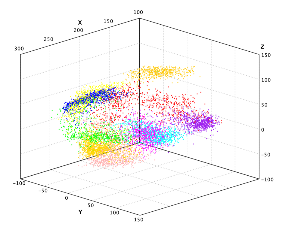
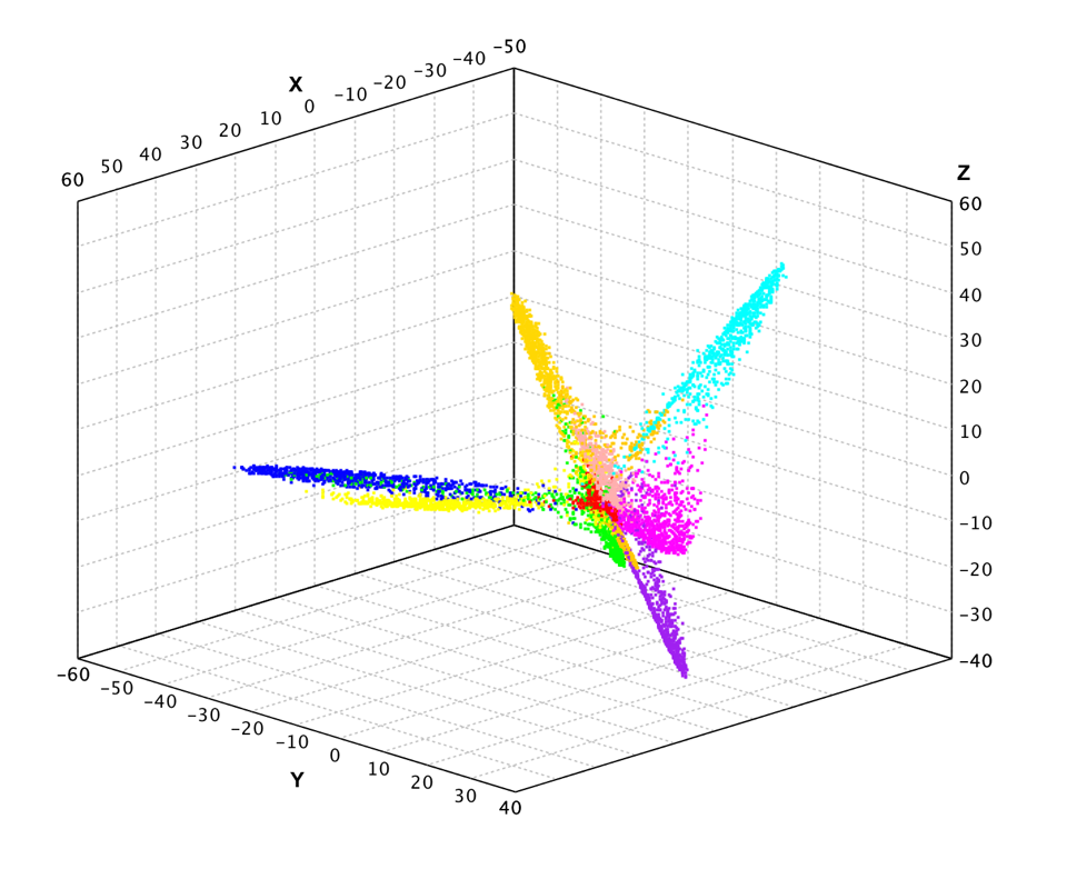
In the above example, we apply PCA to the pen-digits data, which includes 16 variables.
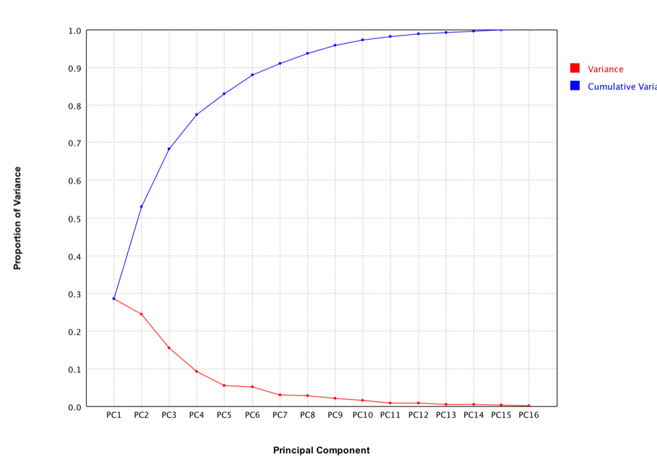
The scree plot is a useful visual aid for determining an appropriate number of principal components. The scree plot graphs the eigenvalue against the component number. To determine the appropriate number of components, we look for an "elbow" in the scree plot. The component number is taken to be the point at which the remaining eigenvalues are relatively small and all about the same size.
Finally, we plot the data projected into 3-dimensional space.

Probabilistic Principal Component Analysis
Probabilistic principal component analysis is a simplified factor analysis that employs a latent variable model with linear relationship:
y ∼ W * x + μ + ε
where latent variables x ∼ N(0, I), error (or noise) ε ∼ N(0, Ψ), and μ is the location term (mean). In probabilistic PCA, an isotropic noise model is used, i.e., noise variances constrained to be equal (Ψi = σ2). A close form of estimation of above parameters can be obtained by maximum likelihood method.
def ppca(data: Array[Array[Double]], k: Int): PPCA
    public class PPCA {
        public static PPCA fit(double[][] data, int k);
    }
Similar to PCA example, we apply probabilistic PCA to the pen-digits data.
    val pc = ppca(df, 3)
    val x2 = pc(x)
    show(plot(x2, y, '.'))
    var pca = ProbabilisticPCA.fit(x, 3);
    var x2 = pca.apply(x);
    ScatterPlot.of(x2, y, '.').canvas().window();
Kernel Principal Component Analysis
Principal component analysis can be employed in a nonlinear way by means of the kernel trick. The resulting technique is capable of constructing nonlinear mappings that maximize the variance in the data. The resulting technique is entitled Kernel PCA. Other prominent nonlinear techniques include manifold learning techniques such as locally linear embedding (LLE), Hessian LLE, Laplacian eigenmaps, and LTSA. These techniques construct a low-dimensional data representation using a cost function that retains local properties of the data, and can be viewed as defining a graph-based kernel for Kernel PCA.
In practice, a large data set leads to a large Kernel/Gram matrix K, and
storing K may become a problem. One way to deal with this is to perform
clustering on your large dataset, and populate the kernel with the means
of those clusters. Since even this method may yield a relatively large K,
it is common to compute only the top P eigenvalues and eigenvectors of K.
def kpca[T](data: Array[T], kernel: MercerKernel[T], k: Int, threshold: Double = 0.0001): KPCA[T]
    public class KPCA {
        public static KPCA<T> fit(T[] data, MercerKernel<T> kernel, int k, double threshold);
    }
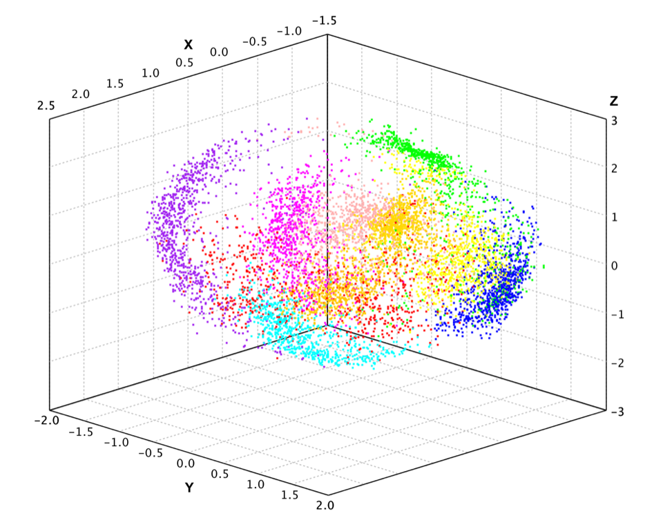
Here we apply kernel PCA to the pen-digits data.
    val pc = kpca(df, new GaussianKernel(45), 3)
    val x2 = pc(x)
    show(plot(x2, y, '.'))
    var pca = KernelPCA.fit(pendigits.drop("V17"), new GaussianKernel(45), 3);
    var x2 = pca.apply(x);
    ScatterPlot.of(x2, y, '.').canvas().window();
Because of its nonlinear nature, the projected data has very different structure from PCA.
Generalized Hebbian Algorithm
Compared to regular batch PCA algorithm, the generalized Hebbian algorithm (GHA) is an adaptive method to find the largest k eigenvectors of the covariance matrix, assuming that the associated eigenvalues are distinct. GHA works with an arbitrarily large sample size and the storage requirement is modest. Another attractive feature is that, in a nonstationary environment, it has an inherent ability to track gradual changes in the optimal solution in an inexpensive way.
It guarantees that GHA finds the first k eigenvectors of the covariance matrix, assuming that the associated eigenvalues are distinct. The convergence theorem is formulated in terms of a time-varying learning rate η. In practice, the learning rate η is chosen to be a small constant, in which case convergence is guaranteed with mean-squared error in synaptic weights of order η.
It also has a simple and predictable trade-off between learning speed and accuracy of convergence as set by the learning rate parameter η. It was shown that a larger learning rate η leads to faster convergence and larger asymptotic mean-square error, which is intuitively satisfying.
    def gha(data: Array[Array[Double]], k: Int, r: Double): GHA

    def gha(data: Array[Array[Double]], w: Array[Array[Double]], r: Double): GHA
    public class GHA {
        public GHA(int n, int p, double r);
        public double update(double[] x);
    }
The first method starts with random initial projection matrix, while the second one starts with a given projection matrix.
    val pc = gha(x, 3, TimeFunction.constant(0.00001))
    val x2 = pc(x)
    show(plot(x2, y, '.'))
    var gha = new GHA(x[0].length, 3, TimeFunction.constant(0.00001));
    Arrays.stream(x).forEach(xi -> gha.update(xi));
    var x2 = gha.apply(x);
    ScatterPlot.of(x2, y, '.').canvas().window();
The results look similar to PCA.