
Classification
The smile.classification
package provides a comprehensive suite of supervised classifiers with a consistent Java API.
This page focuses on practical Java usage patterns and algorithm-specific examples.
API Overview
- Most models are trained through static
fit(...)factory methods. - Class labels may be arbitrary integers (for example
-1/+1or3/7/14). - All classifiers implement
Classifier<T>. - Models are serializable and many support
Properties-based hyperparameter configuration.
Each model has an inner Options record class to define hyperparameters
in strongly typed approach. Meanwhile, the Properties-based configuration
is convenient for reproducible, configuration-file-driven workflows.
    Properties params = new Properties();
    params.setProperty("smile.random.forest.trees", "200");
    params.setProperty("smile.random.forest.max.depth", "10");

    RandomForest model = RandomForest.fit(formula, data, params);
The central API supports hard prediction, optional probabilities, optional raw scores, and optional online updates. Before using a classifier, it is useful to check whether the model supports soft prediction or online updates.
    // Works for any smile.classification.Classifier<T>
    int label = model.predict(sample);

    if (model.isSoft()) {
        double[] posteriori = new double[model.numClasses()];
        model.predict(sample, posteriori); // class probabilities
    }

    if (model.isOnline()) {
        model.update(newSample, newLabel); // incremental learning
    }
DataFrameClassifier
Many models (e.g., tree-based ones) operate on DataFrame inputs with
a Formula and implement DataFrameClassifier.
    Formula formula = Formula.lhs("species");
    DecisionTree tree = DecisionTree.fit(formula, data);
    int[] labels = tree.predict(data);
Class Label Handling
SMILE internally remaps labels to contiguous indices and returns original labels at prediction time.
    int[] y = {-1, +1, -1, +1};
    LogisticRegression model = LogisticRegression.fit(x, y);
    int label = model.predict(sample);   // returns -1 or +1
Quick Algorithm Selection Guide
There is no universally the best classifier. Use the table below as a starting point.
| Situation | Recommended Models | Notes |
|---|---|---|
| Strong default baseline | RandomForest |
Robust with mixed tabular features; supports OOB error estimates. |
| Highest tuned accuracy on tabular data | GradientTreeBoost |
Usually strongest after tuning, but more sensitive to hyperparameters. |
| Fast, interpretable model | DecisionTree, LogisticRegression |
Good for explainability and quick diagnostics. |
| Very high-dimensional sparse text/features | DiscreteNaiveBayes, SparseLogisticRegression, Maxent |
Designed for sparse count-style inputs. |
More features than samples (p > n) |
FLD, SparseLogisticRegression |
Avoid plain LDA/QDA in this regime due to covariance instability. |
| Streaming / incremental updates | LogisticRegression, DiscreteNaiveBayes, MLP |
Check isOnline() before calling update. |
Algorithm Comparison
| Algorithm | Input | isSoft | isOnline | DataFrame | Typical Use |
|---|---|---|---|---|---|
| LDA / QDA / RDA / FLD | double[] |
Mostly yes (FLD no) | No | No | Classical Gaussian discriminant models |
| LogisticRegression / SparseLogisticRegression / Maxent | double[], SparseArray, int[] |
Yes | Yes | No | Linear baselines and sparse NLP classification |
| DecisionTree / RandomForest / AdaBoost / GradientTreeBoost | Tuple via Formula |
Yes | No | Yes | General-purpose tabular learning |
| KNN / RBFNetwork | Generic T |
KNN yes, RBFNetwork no | No | No | Instance-based / local nonlinear boundaries |
| SVM / LinearSVM | Generic T or linear vectors |
Score-based (not posterior by default) | No | No | Max-margin classification, often with OVO/OVR |
| MLP | double[] |
Yes | Yes | No | Nonlinear expressive models |
Practical Tips
- Scale-sensitive models include KNN, SVM, logistic regression, MLP, and discriminant analysis.
- Tree-based models are mostly scale-invariant and usually easiest to start with on mixed tabular data.
- Set a random seed for reproducibility when training stochastic models.
- Persist trained models with
smile.io.Write/smile.io.Read.
    smile.math.MathEx.setSeed(12345);

    Write.object(model, Path.of("classifier.sml"));
    Classifier<?> loaded = (Classifier<?>) Read.object(Path.of("classifier.sml"));
Background
In machine learning and pattern recognition, classification refers to an algorithmic procedure for assigning a given input object into one of a given number of categories. The input object is formally termed an instance, and the categories are termed classes.
The instance is usually described by a vector of features, which together constitute a description of all known characteristics of the instance. Typically, features are either categorical (also known as nominal, i.e. consisting of one of a set of unordered items, such as a gender of "male" or "female", or a blood type of "A", "B", "AB" or "O"), ordinal (consisting of one of a set of ordered items, e.g. "large", "medium" or "small"), integer-valued (e.g. a count of the number of occurrences of a particular word in an email) or real-valued (e.g. a measurement of blood pressure).
Classification normally refers to a supervised procedure, i.e. a procedure that produces an inferred function to predict the output value of new instances based on a training set of pairs consisting of an input object and a desired output value. The inferred function is called a classifier if the output is discrete or a regression function if the output is continuous.
The inferred function should predict the correct output value for any valid input object. This requires the learning algorithm to generalize from the training data to unseen situations in a "reasonable" way.
A wide range of supervised learning algorithms is available, each with its strengths and weaknesses. There is no single learning algorithm that works best on all supervised learning problems. The most widely used learning algorithms are AdaBoost and gradient boosting, support vector machines, linear regression, linear discriminant analysis, logistic regression, naive Bayes, decision trees, k-nearest neighbor algorithm, and neural networks (multilayer perceptron).
If the feature vectors include features of many different kinds (discrete, discrete ordered, counts, continuous values), some algorithms cannot be easily applied. Many algorithms, including linear regression, logistic regression, neural networks, and nearest neighbor methods, require that the input features be numerical and scaled to similar ranges (e.g., to the [-1,1] interval). Methods that employ a distance function, such as nearest neighbor methods and support vector machines with Gaussian kernels, are particularly sensitive to this. An advantage of decision trees (and boosting algorithms based on decision trees) is that they easily handle heterogeneous data.
If the input features contain redundant information (e.g., highly correlated features), some learning algorithms (e.g., linear regression, logistic regression, and distance based methods) will perform poorly because of numerical instabilities. These problems can often be solved by imposing some form of regularization.
If each of the features makes an independent contribution to the output, then algorithms based on linear functions (e.g., linear regression, logistic regression, linear support vector machines, naive Bayes) generally perform well. However, if there are complex interactions among features, then algorithms such as nonlinear support vector machines, decision trees and neural networks work better. Linear methods can also be applied, but the engineer must manually specify the interactions when using them.
There are several major issues to consider in supervised learning:
- Features
The accuracy of the inferred function depends strongly on how the input object is represented. Typically, the input object is transformed into a feature vector, which contains a number of features that are descriptive of the object. The number of features should not be too large, because of the curse of dimensionality; but should contain enough information to accurately predict the output.
There are many algorithms for feature selection that seek to identify the relevant features and discard the irrelevant ones. More generally, dimensionality reduction may seek to map the input data into a lower dimensional space prior to running the supervised learning algorithm.
- Overfitting
Overfitting occurs when a statistical model describes random error or noise instead of the underlying relationship. Overfitting generally occurs when a model is excessively complex, such as having too many parameters relative to the number of observations. A model which has been overfit will generally have poor predictive performance, as it can exaggerate minor fluctuations in the data.
The potential for overfitting depends not only on the number of parameters and data but also the conformability of the model structure with the data shape, and the magnitude of model error compared to the expected level of noise or error in the data.
In order to avoid overfitting, it is necessary to use additional techniques (e.g. cross-validation, regularization, early stopping, pruning, Bayesian priors on parameters or model comparison), that can indicate when further training is not resulting in better generalization. The basis of some techniques is either (1) to explicitly penalize overly complex models, or (2) to test the model's ability to generalize by evaluating its performance on a set of data not used for training, which is assumed to approximate the typical unseen data that a model will encounter.
- Regularization
Regularization involves introducing additional information in order to solve an ill-posed problem or to prevent over-fitting. This information is usually of the form of a penalty for complexity, such as restrictions for smoothness or bounds on the vector space norm. A theoretical justification for regularization is that it attempts to impose Occam's razor on the solution. From a Bayesian point of view, many regularization techniques correspond to imposing certain prior distributions on model parameters.
- Bias-variance tradeoff
Mean squared error (MSE) can be broken down into two components: variance and squared bias, known as the bias-variance decomposition. Thus, in order to minimize the MSE, we need to minimize both the bias and the variance. However, this is not trivial. Therefore, there is a tradeoff between bias and variance.
K-Nearest Neighbor
The k-nearest neighbor algorithm (k-NN) is a method for classifying objects by a majority vote of its neighbors, with the object being assigned to the class most common amongst its k nearest neighbors (k is typically small). k-NN is a type of instance-based learning, or lazy learning where the function is only approximated locally and all computation is deferred until classification.
def knn(x: Array[Array[Double]], y: Array[Int], k: Int): KNN[Array[Double]]
    public class KNN {
        public static KNN<double[]> fit(double[][] x, int[] y, int k);
    }
fun knn(x: Array<DoubleArray>, y: IntArray, k: Int): KNN<DoubleArray>
The simplest k-NN method takes a data set of feature vectors and labels
with Euclidean distance as the similarity measure. When applied to the
Iris dataset, the accuracy of 10-fold cross validation is 96% for k = 3.
    val iris = read.arff("data/weka/iris.arff")
    val x = iris.drop("class").toArray()
    val y = iris("class").toIntArray()
    cv.classification(10, x, y) { case (x, y) => knn(x, y, 3) }
    var iris = Read.arff("data/weka/iris.arff");
    var x = iris.drop("class").toArray();
    var y = iris.column("class").toIntArray();
    CrossValidation.classification(10, x, y, (x, y) -> KNN.fit(x, y, 3));
    val iris = read.arff("data/weka/iris.arff")
    val x = iris.drop("class").toArray()
    val y = iris.column("class").toIntArray()
    CrossValidation.classification(10, x, y, {x, y -> KNN.fit(x, y, 3)})
The best choice of k depends upon the data; generally, larger values of k reduce the effect of noise on the classification, but make boundaries between classes less distinct. A good k can be selected by various heuristic techniques, e.g. cross-validation. In binary problems, it is helpful to choose k to be an odd number as this avoids tied votes.
The nearest neighbor algorithm has some strong consistency results. As the amount of data approaches infinity, the algorithm is guaranteed to yield an error rate no worse than twice the Bayes error rate (the minimum achievable error rate given the distribution of the data). k-NN is guaranteed to approach the Bayes error rate, for some value of k (where k increases as a function of the number of data points).
The user can also provide a customized distance function.
def knn[T](x: Array[T], y: Array[Int], k: Int, distance: Distance[T]): KNN[T]
    public class KNN {
        public static KNN<T> fit(T[] x, int[] y, int k, Distance<T> distance);
    }
fun <T> knn(x: Array<T>, y: IntArray, k: Int, distance: Distance<T>): KNN<T>
Often, the classification accuracy of k-NN can be improved significantly if the distance metric is learned with specialized algorithms such as Large Margin Nearest Neighbor or Neighborhood Components Analysis.
Alternatively, the user may provide a k-nearest neighbor search data structure. Besides the simple linear search, SMILE provides KD-Tree, Cover Tree, and LSH (Locality-Sensitive Hashing) for efficient k-nearest neighbor search.
def knn[T](x: KNNSearch[T, T], y: Array[Int], k: Int): KNN[T]
    public class KNN {
        public KNN(KNNSearch<T, T> knn, int[] y, int k);
    }
fun <T> knn(x: KNNSearch<T, T>, y: IntArray, k: Int): KNN<T>
A KD-tree (short for k-dimensional tree) is a space-partitioning dataset structure for organizing points in a k-dimensional space. Cover tree is a data structure for generic nearest neighbor search (with a metric), which is especially efficient in spaces with small intrinsic dimension. The cover tree has a theoretical bound that is based on the dataset's doubling constant. LSH is an efficient algorithm for approximate nearest neighbor search in high dimensional spaces by performing probabilistic dimension reduction of data.
Nearest neighbor rules in effect compute the decision boundary in an
implicit manner. In the following example, we show the implicit decision
boundary of k-NN on a 2-dimensional toy data. Please try different k,
and you will observe the change of decision boundary. In general, the larger
k, the smoother the boundary.
    val toy = read.csv("data/classification/toy200.txt", delimiter="\t", header=false)
    val x = toy.select(1, 2).toArray()
    val y = toy.column(0).toIntArray()
    knn(x, y, 3)
    var toy = Read.csv("data/classification/toy200.txt", CSVFormat.DEFAULT.withDelimiter('\t'));
    var x = toy.select(1, 2).toArray();
    var y = toy.column(0).toIntArray();
    KNN.fit(x, y, 3);
    import smile.*;
    import smile.classification.*;
    val toy = read.csv("data/classification/toy200.txt", delimiter='\t', header=false)
    val x = toy.select(1, 2).toArray()
    val y = toy.column(0).toIntArray()
    knn(x, y, 3)
In what follows, we will discuss the classification methods that compute the decision boundary explicitly. The computational complexity in the prediction phase is therefore a function of the boundary complexity. We will start with the simplest linear decision functions.
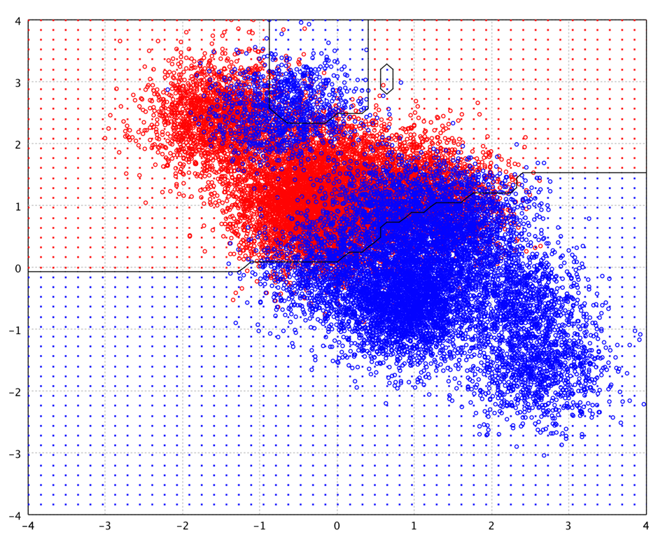
Linear Discriminant Analysis
Linear discriminant analysis (LDA) is based on the Bayes decision theory and assumes that the conditional probability density functions are normally distributed. LDA also makes the simplifying homoscedastic assumption (i.e. that the class covariances are identical) and that the covariances have full rank. With these assumptions, the discriminant function of an input being in a class is purely a function of this linear combination of independent variables.
def lda(x: Array[Array[Double]], y: Array[Int], priori: Array[Double] = null, tol: Double = 0.0001):LDA
    public class LDA {
        public static LDA fit(double[][] x, int[] y, double[] priori, double tol);
    }
fun lda(x: Array<DoubleArray>, y: IntArray, priori: DoubleArray? = null, tol: Double = 0.0001): LDA
The parameter priori is the priori probability of each class. If null, it will be
estimated from the training data. The parameter tol is a tolerance to decide
if a covariance matrix is singular. The function will reject variables whose variance is
less than tol2.
lda(x, y)
LDA.fit(x, y);
lda(x, y)
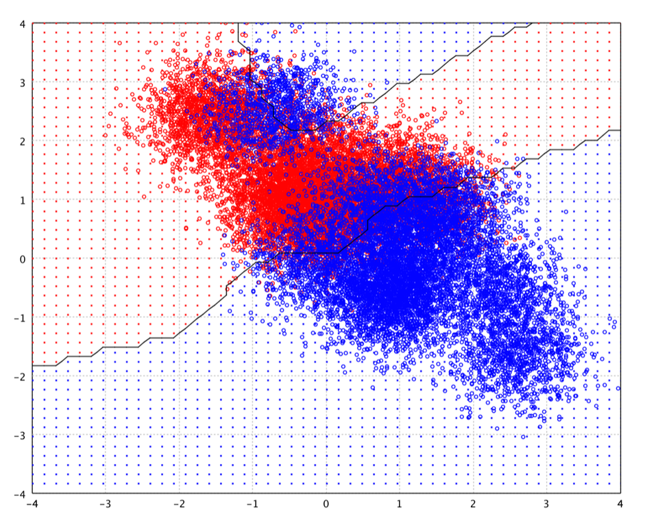
As shown in the plot of toy data, the decision boundary of LDA is linear. Note that the decision boundary in the plot is the estimated contour on the testing grid (small dots) rather than the exact decision function. Therefore, there are the artifacts caused by discretized grid.
LDA is closely related to ANOVA (analysis of variance) and linear regression analysis, which also attempt to express one dependent variable as a linear combination of other features or measurements. In the other two methods, however, the dependent variable is a numerical quantity, while for LDA it is a categorical variable (i.e. the class label). Logistic regression and probit regression are more similar to LDA, as they also explain a categorical variable. These other methods are preferable in applications where it is not reasonable to assume that the independent variables are normally distributed, which is a fundamental assumption of the LDA method.
One complication in applying LDA (and Fisher's discriminant) to real data occurs when the number of variables/features does not exceed the number of samples. In this case, the covariance estimates do not have full rank, and so cannot be inverted. This is known as small sample size problem.
Fisher's Linear Discriminant
Fisher's linear discriminant (FLD) is another popular linear classifier. Fisher defined the separation between two distributions to be the ratio of the variance between the classes to the variance within the classes, which is, in some sense, a measure of the signal-to-noise ratio for the class labeling. FLD finds a linear combination of features which maximizes the separation after the projection. The resulting combination may be used for dimensionality reduction before later classification.
def fisher(x: Array[Array[Double]], y: Array[Int], L: Int = -1, tol: Double = 0.0001): FLD
    public class FLD {
        public static FLD fit(double[][] x, int[] y, int L, double tol);
    }
fun fisher(x: Array<DoubleArray>, y: IntArray, L: Int = -1, tol: Double = 0.0001): FLD
The parameter L is the dimensionality of mapped space.
The default value is the number of classes - 1.
In FLD, the features are mapped to the subspace spanned by the eigenvectors
corresponding to the C − 1 largest eigenvalues of
Σ-1Σb,
where Σ is the covariance matrix,
Σb is the scatter matrix between class means,
and C is the number of classes.
The terms Fisher's linear discriminant and LDA are often used interchangeably, although FLD actually describes a slightly different discriminant, which does not make some of the assumptions of LDA such as normally distributed classes or equal class covariances. When the assumptions of LDA are satisfied, FLD is equivalent to LDA.
fisher(x, y)
FLD.fit(x, y);
fisher(x, y)

FLD is also closely related to principal component analysis (PCA), which also looks for linear combinations of variables which best explain the data. As a supervised method, FLD explicitly attempts to model the difference between the classes of data. On the other hand, PCA is an unsupervised method and does not take into account any difference in class.
One complication in applying FLD (and LDA) to real data occurs when the number of variables/features does not exceed the number of samples. In this case, the covariance estimates do not have full rank, and so cannot be inverted. This is known as small sample size problem.
Quadratic Discriminant analysis
Quadratic discriminant analysis (QDA) is closely related to LDA. Like LDA, QDA models the conditional probability density functions as a Gaussian distribution, then uses the posterior distributions to estimate the class for a given test data.
def qda(x: Array[Array[Double]], y: Array[Int], priori: Array[Double] = null, tol: Double = 0.0001):QDA
    public class QDA {
        public static QDA fit(double[][] x, int[] y, double[] priori, double tol);
    }
fun qda(x: Array<DoubleArray>, y: IntArray, priori: DoubleArray? = null, tol: Double = 0.0001): QDA
Unlike LDA, however, in QDA there is no assumption that the covariance of each of the classes is identical. Therefore, the resulting separating surface between the classes is quadratic.
qda(x, y)
QDA.fit(x, y);
qda(x, y)
The Gaussian parameters for each class can be estimated from training data with maximum likelihood (ML) estimation. However, when the number of training instances is small compared to the dimension of input space, the ML covariance estimation can be ill-posed. One approach to resolve the ill-posed estimation is to regularize the covariance estimation as in regularized discriminant analysis.
Regularized Discriminant Analysis
In LDA and FLD, the eigenvectors corresponding to the smaller eigenvalues will tend to be very sensitive to the exact choice of training data, and it is often necessary to use regularization. In the regularized discriminant analysis (RDA), the regularized covariance matrices of each class is Σk(α) = α Σk + (1 - α) Σ.
def rda(x: Array[Array[Double]], y: Array[Int], alpha: Double, priori: Array[Double] = null, tol: Double = 0.0001): RDA
    public class RDA {
        public static RDA fit(double[][] x, int[] y, double alpha, double[] priori, double tol);
    }
fun rda(x: Array<DoubleArray>, y: IntArray, alpha: Double, priori: DoubleArray? = null, tol: Double = 0.0001): RDA
where the parameter alpha is the regularization factor in [0, 1].
RDA is a compromise between LDA and QDA, which allows one to shrink the separate covariances of QDA toward a common variance as in LDA. This method is very similar in flavor to ridge regression. The quadratic discriminant function is defined using the shrunken covariance matrices Σk(α). The parameter α in [0, 1] controls the complexity of the model. When α is one, RDA becomes QDA. While α is zero, RDA is equivalent to LDA. Therefore, the regularization factor α allows a continuum of models between LDA and QDA.
rda(x, y, 0.1)
RDA.fit(x, y, 0.1);
rda(x, y, 0.1)
Logistic Regression
Logistic regression (logit model) is a generalized linear model used for binomial regression. Logistic regression applies maximum likelihood estimation after transforming the dependent into a logit variable. A logit is the natural log of the odds of the dependent equaling a certain value or not (usually 1 in binary logistic models, the highest value in multinomial models). In this way, logistic regression estimates the odds of a certain event (value) occurring.
    def logit(x: Array[Array[Double]],
              y: Array[Int],
              lambda: Double = 0.0,
              tol: Double = 1E-5,
              maxIter: Int = 500): LogisticRegression
    public class LogisticRegression {
        public static LogisticRegression fit(double[][] x, int[] y, Options options);
    }
    fun logit(x: Array<DoubleArray>,
              y: IntArray,
              lambda: Double = 0.0,
              tol: Double = 1E-5,
              maxIter: Int = 500): LogisticRegression
where the parameter lambda (> 0) gives a "regularized" estimate of linear
weights which often has superior generalization performance, especially
when the dimensionality is high.
logit(x, y)
LogisticRegression.fit(x, y);
logit(x, y)

Logistic regression has many analogies to ordinary least squares (OLS) regression. Unlike OLS regression, however, logistic regression does not assume linearity of relationship between the raw values of the independent variables and the dependent, does not require normally distributed variables, does not assume homoscedasticity, and in general has less stringent requirements.
Compared with linear discriminant analysis, logistic regression has several advantages:
- It is more robust: the independent variables don't have to be normally distributed, or have equal variance in each group
- It does not assume a linear relationship between the independent variables and dependent variable.
- It may handle nonlinear effects since one can add explicit interaction and power terms.
However, it requires much more data to achieve stable, meaningful results.
Logistic regression also has strong connections with neural network and maximum entropy modeling. For example, binary logistic regression is equivalent to a one-layer, single-output neural network with a logistic activation function trained under log loss. Similarly, multinomial logistic regression is equivalent to a one-layer, softmax-output neural network.
Logistic regression estimation also obeys the maximum entropy principle, and thus logistic regression is sometimes called "maximum entropy modeling", and the resulting classifier the "maximum entropy classifier".
Maximum Entropy Classifier
Maximum entropy is a technique for learning probability distributions from data. In maximum entropy models, the observed data itself is assumed to be the testable information. Maximum entropy models don't assume anything about the probability distribution other than what have been observed and always choose the most uniform distribution subject to the observed constraints.
    def maxent(x: Array[Array[Int]],
               y: Array[Int],
               p: Int,
               lambda: Double = 0.1,
               tol: Double = 1E-5,
               maxIter: Int = 500): Maxent
    public class Maxent {
        public static Maxent fit(int[][] x, int[] y, Options options);
    }
    fun maxent(x: Array<IntArray>,
               y: IntArray,
               p: Int,
               lambda: Double = 0.1,
               tol: Double = 1E-5,
               maxIter: Int = 500): Maxent
where x is the sparse training samples. Each sample is represented by a set of sparse
binary features. The features are stored in an integer array, of which
are the indices of nonzero features.
The parameter p is the dimension of feature space, and lambda
is the regularization factor.
Basically, maximum entropy classifier is another name of multinomial logistic regression applied to categorical independent variables, which are converted to binary dummy variables. Maximum entropy models are widely used in natural language processing. Therefore, our implementation assumes that binary features are stored in a sparse array, of which entries are the indices of nonzero features.
Multilayer Perceptron Neural Network
A multilayer perceptron neural network consists of several layers of nodes, interconnected through weighted acyclic arcs from each preceding layer to the following, without lateral or feedback connections. Each node calculates a transformed weighted linear combination of its inputs (output activations from the preceding layer), with one of the weights acting as a trainable bias connected to a constant input. The transformation, called activation function, is a bounded non-decreasing (non-linear) function, such as the sigmoid functions (ranges from 0 to 1). Another popular activation function is hyperbolic tangent which is actually equivalent to the sigmoid function in shape but ranges from -1 to 1. More specialized activation functions include radial basis functions which are used in RBF networks.
For neural networks, the input patterns usually should be scaled/standardized. Commonly, each input variable is scaled into interval [0, 1] or to have mean 0 and standard deviation 1.
    def mlp(x: Array[Array[Double]],
            y: Array[Int],
            builders: Array[LayerBuilder],
            epochs: Int = 10,
            learningRate: TimeFunction = TimeFunction.linear(0.01, 10000, 0.001),
            momentum: TimeFunction = TimeFunction.constant(0.0),
            weightDecay: Double = 0.0,
            rho: Double = 0.0,
            epsilon: Double = 1E-7): MLP
    public class MLP {
        public MLP(int p, LayerBuilder... builders);
    }
    fun mlp(x: Array<DoubleArray>,
            y: IntArray,
            builders: Array<LayerBuilder>,
            epochs: Int = 10,
            learningRate: TimeFunction = TimeFunction.linear(0.01, 10000.0, 0.001),
            momentum: TimeFunction = TimeFunction.constant(0.0),
            weightDecay: Double = 0.0,
            rho: Double = 0.0,
            epsilon: Double = 1E-7): MLP
where p is the number of input variables, builders
defines each layer of network,
epochs is the number of epochs of stochastic learning,
eta is the learning rate,
alpha is the momentum factor,
and lambda is the weight decay for regularization.
The meaning of these parameters will be clear in the following discussion.
For error/penalty functions and output units, the following natural pairings are recommended:
- linear output units and least squares penalty function.
- a two-class cross-entropy penalty function and a logistic activation function.
- a multi-class cross-entropy penalty function and a softmax activation function.
By assigning a softmax activation function on the output layer of the neural network for categorical target variables, the outputs can be interpreted as posterior probabilities, which are very useful.
    val net = mlp(x, y, Array(Layer.input(2), Layer.sigmoid(10), Layer.mle(1, OutputFunction.SIGMOID)),
        learningRate = TimeFunction.constant(0.1), momentum = TimeFunction.constant(0.1))
    import smile.base.mlp.*;
    var net = new MLP(Layer.input(2),
                Layer.sigmoid(10),
                Layer.mle(1, OutputFunction.SIGMOID)
            );

    net.setLearningRate(TimeFunction.constant(0.1));
    net.setMomentum(TimeFunction.constant(0.1));

    for (int epoch = 0; epoch < 10; epoch++) {
        for (int i : MathEx.permutate(x.length)) {
            net.update(x[i], y[i]);
        }
    }
    import smile.base.mlp.*
    import smile.math.*;
    mlp(x, y, arrayOf(Layer.input(2), Layer.sigmoid(10), Layer.mle(1, OutputFunction.SIGMOID)),
        learningRate = TimeFunction.constant(0.1), momentum = TimeFunction.constant(0.1))
The representational capabilities of a neural network are determined by the range of mappings it may implement through weight variation. Single layer perceptrons are capable of solving only linearly separable problems. With the sigmoid function as activation function, the single-layer network is identical to the logistic regression model.
The universal approximation theorem for neural networks states that every continuous function that maps intervals of real numbers to some output interval of real numbers can be approximated arbitrarily closely by a multi-layer perceptron with just one hidden layer. This result holds only for restricted classes of activation functions, which are extremely complex and NOT smooth for subtle mathematical reasons. On the other hand, smoothness is important for gradient descent learning. Besides, the proof is not constructive regarding the number of neurons required or the settings of the weights. Therefore, complex systems will have more layers of neurons with some having increased layers of input neurons and output neurons in practice. The extra layers enable composition of features from lower layers, giving the potential of modeling complex data with fewer units than a similarly performing shallow network. But many issues can arise with deep neural networks if they are naively trained. Two common issues are overfitting and computation time.
The most popular algorithm to train neural networks is back-propagation, which is a gradient descent method. Based on chain rule, the algorithm propagates the error back through the network and adjusts the weights of each connection in order to reduce the value of the error function by some small amount. For this reason, back-propagation can only be applied on networks with differentiable activation functions.
During error back propagation, we usually times the gradient with a small number η, called learning rate, which is carefully selected to ensure that the network converges to a local minimum of the error function fast enough, without producing oscillations. One way to avoid oscillation at large η, is to make the change in weight dependent on the past weight change by adding a momentum term.
Although the back-propagation algorithm may perform gradient descent on the total error of all instances in a batch way, the learning rule is often applied to each instance separately in an online way or stochastic way. There exists empirical indication that the stochastic way results in faster convergence.
In practice, the problem of over-fitting has emerged. This arises in convoluted or over-specified systems when the capacity of the network significantly exceeds the needed free parameters. There are two general approaches for avoiding this problem: The first is to use cross-validation and similar techniques to check for the presence of over-fitting and optimally select hyperparameters such as to minimize the generalization error. The second is to use some form of regularization, which emerges naturally in a Bayesian framework, where the regularization can be performed by selecting a larger prior probability over simpler models; but also in statistical learning theory, where the goal is to minimize over the "empirical risk" and the "structural risk".
Radial Basis Function Networks
A radial basis function network is an artificial neural network that uses radial basis functions as activation functions. It is a linear combination of radial basis functions. They are used in function approximation, time series prediction, and control.
In its basic form, radial basis function network is in the form
y(x) = Σ wi φ(||x-ci||)
where the approximating function y(x) is represented as a sum of N radial basis functions φ, each associated with a different center ci, and weighted by an appropriate coefficient wi. For distance, one usually chooses Euclidean distance. The weights wi can be estimated using the matrix methods of linear least squares, because the approximating function is linear in the weights.
RBF networks are typically trained by a two-step algorithm.
In the first step, the center vectors ci
of the RBF functions in the hidden layer are chosen.
This step can be performed in several ways; centers can be randomly
sampled from some set of examples, or they can be determined
using k-means clustering. Note that this step is unsupervised.
The second step simply fits a linear model with coefficients wi to
the hidden layer's outputs with respect to some objective function.
A common objective function, at least for regression/function estimation,
is the least squares function.
An optional third backpropagation step can be performed to fine-tune all the RBF network's parameters.
def rbfnet[T](x: Array[T], y: Array[Int], neurons: Array[RBF[T]], normalized: Boolean): RBFNetwork[T]
    public class RBFNetwork {
        public static RBFNetwork<T> fit(T[] x, int[] y, RBF<T>[] rbf, boolean normalized);
    }
fun <T> rbfnet(x: Array<T>, y: IntArray, neurons: Array<RBF<T>>, normalized: Boolean = false): RBFNetwork<T>
The popular choices for φ comprise the Gaussian function and the so-called thin plate splines. The advantage of the thin plate splines is that their conditioning is invariant under scalings. Gaussian, multi-quadric and inverse multi-quadric are infinitely smooth and involve a scale or shape parameter, r0 > 0. Decreasing r0 tends to flatten the basis function. For a given function, the quality of approximation may strongly depend on this parameter. In particular, increasing r0 has the effect of better conditioning (the separation distance of the scaled points increases).
val rbf = rbfnet(x, y, RBF.fit(x, 50), false)
    import smile.base.rbf.*;
    RBFNetwork.fit(x, y, RBF.fit(x, 50), false);
    import smile.base.rbf.*
    rbfnet(x, y, RBF.fit(x, 50), false)
After running the above example, you may notice that the decision boundary
may be very different from the below picture. It is because the centers
learn from gaussrbf, employing K-Means in this example,
are different every time, a nature of stochastic algorithm like K-Means.
This also shows that the decision boundary of RBF network is very sensistive
to the chosen centers.
A variant on RBF networks is normalized radial basis function (NRBF) networks, in which we require the sum of the basis functions to be unity. NRBF arises more naturally from a Bayesian statistical perspective. However, there is no evidence that either the NRBF method is consistently superior to the RBF method, or vice versa.
Support Vector Machines
The basic support vector machine (SVM) is a binary linear classifier which chooses the hyperplane that represents the largest separation, or margin, between the two classes. If such a hyperplane exists, it is known as the maximum-margin hyperplane and the linear classifier it defines is known as a maximum margin classifier.
If there exists no hyperplane that can perfectly split the positive and negative instances, the soft margin method will choose a hyperplane that splits the instances as cleanly as possible, while still maximizing the distance to the nearest cleanly split instances.
The nonlinear SVMs are created by applying the kernel trick to maximum-margin hyperplanes. The resulting algorithm is formally similar, except that every dot product is replaced by a nonlinear kernel function. This allows the algorithm to fit the maximum-margin hyperplane in a transformed feature space. The transformation may be nonlinear and the transformed space be high dimensional. For example, the feature space corresponding Gaussian kernel is a Hilbert space of infinite dimension. Thus, though the classifier is a hyperplane in the high-dimensional feature space, it may be nonlinear in the original input space. Maximum margin classifiers are well regularized, so the infinite dimension does not spoil the results.
def svm[T <](x: Array[T], y: Array[Int], kernel: MercerKernel[T], C: Double, tol: Double = 1E-3): SVM[T]
    public class SVM {
        // Fits a binary-class linear SVM
        public static Classifier<double[]> fit(double[][] x, int[] y, Options options);
        // Fits a binary-class linear SVM of binary sparse data
        public static Classifier<int[]> fit(int[][] x, int[] y, int p, Options options);
        // Fits a binary-class linear SVM of binary sparse data
        public static Classifier<SparseArray> fit(SparseArray[] x, int[] y, int p, Options options);
        // Fits a non-linear SVM
        public static SVM<T> fit(T[] x, int[] y, MercerKernel<T> kernel, Options options);
    }
fun <T> svm(x: Array<T>, y: IntArray, kernel: MercerKernel<T>, C: Double, tol: Double = 1E-3): SVM<T>
The effectiveness of SVM depends on the selection of kernel, the kernel's
parameters, and soft margin parameter C. Given a kernel, best combination
of C and kernel's parameters is often selected by a grid-search with
cross validation.
The dominant approach for creating multi-class SVMs is to reduce the single multi-class problem into multiple binary classification problems. Common methods for such reduction is to build binary classifiers which distinguish between (i) one of the labels to the rest (one-versus-rest or one-versus-all) or (ii) between every pair of classes (one-versus-one). Classification of new instances for one-versus-all case is done by a winner-takes-all strategy, in which the classifier with the highest output function assigns the class. For the one-versus-one approach, classification is done by a max-wins voting strategy, in which every classifier assigns the instance to one of the two classes, then the vote for the assigned class is increased by one vote, and finally the class with most votes determines the instance classification.
    // One-vs-one strategy
    def ovo[T](x: Array[T], y: Array[Int])(trainer: (Array[T], Array[Int]) => Classifier[T]): OneVersusOne[T]

    // One-vs-rest (or one-vs-all) strategy
    def ovr[T](x: Array[T], y: Array[Int])(trainer: (Array[T], Array[Int]) => Classifier[T]): OneVersusRest[T]
    public class OneVersusOne {
         public static OneVersusOne<T> fit(T[] x, int[] y, BiFunction<T[], int[], Classifier<T>> trainer);
    }

    public class OneVersusRest {
         public static OneVersusRest<T> fit(T[] x, int[] y, BiFunction<T[], int[], Classifier<T>> trainer);
    }
    // One-vs-one strategy
    fun <T> ovo(x: Array<T>, y: IntArray, trainer: (Array<T>, IntArray) -> Classifier<T>): OneVersusOne<T>

    // One-vs-rest (or one-vs-all) strategy
    fun <T> ovr(x: Array<T>, y: IntArray, trainer: (Array<T>, IntArray) -> Classifier<T>): OneVersusRest<T>
    val zip = read.csv("data/usps/zip.train", delimiter = ' ' , header = false)
    val x = zip.drop(0).toArray()
    val y = zip.column(0).toIntArray()
    val kernel = new GaussianKernel(8.0)
    val model = ovr(x, y) { (x, y) => SVM.fit(x, y, kernel, 5, 1E-3) }
    var zip = Read.csv("data/usps/zip.train", CSVFormat.DEFAULT.withDelimiter(' '));
    var x = zip.drop(0).toArray();
    var y = zip.column(0).toIntArray();
    var kernel = new GaussianKernel(8.0);
    var model = OneVersusRest.fit(x, y, (x, y) -> SVM.fit(x, y, kernel, new SVM.Options(5)));
    val zip = read.csv("data/usps/zip.train", delimiter = ' ' , header = false)
    val x = zip.drop(0).toArray()
    val y = zip.column(0).toIntArray()
    val kernel = GaussianKernel(8.0)
    val model = ovr(x, y, { x, y -> svm(x, y, kernel, 5.0, 1E-3) })
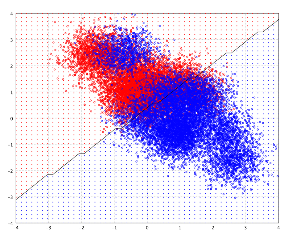
With a Gaussian kernel of γ = 1.0 and C = 10,
the decission boundary of SVM on the toy data is shown as following.
SVMs with Gaussian kernel have similar structure as RBF networks with Gaussian radial basis functions. However, the SVM approach "automatically" solves the network complexity problem since the size of the hidden layer is obtained as the result of the quadratic programming procedure. Hidden neurons and support vectors correspond to each other, so the center problems of the RBF network is also solved, as the support vectors serve as the basis function centers. It was reported that with similar number of support vectors/centers, SVM shows better generalization performance than RBF network when the training data size is relatively small. On the other hand, RBF network gives better generalization performance than SVM on large training data.
Decision Trees
A decision tree can be learned by splitting the training set into subsets based on an attribute value test. This process is repeated on each derived subset in a recursive manner called recursive partitioning. The recursion is completed when the subset at a node all has the same value of the target variable, or when splitting no longer adds value to the predictions.
The algorithms that are used for constructing decision trees usually work top-down by choosing a variable at each step that is the next best variable to use in splitting the set of items. "Best" is defined by how well the variable splits the set into homogeneous subsets that have the same value of the target variable. Different algorithms use different formulae for measuring "best". Used by the CART (Classification and Regression Tree) algorithm, Gini impurity is a measure of how often a randomly chosen element from the set would be incorrectly labeled if it were randomly labeled according to the distribution of labels in the subset. Gini impurity can be computed by summing the probability of each item being chosen times the probability of a mistake in categorizing that item. It reaches its minimum (zero) when all cases in the node fall into a single target category. Information gain is another popular measure, used by the ID3, C4.5 and C5.0 algorithms. Information gain is based on the concept of entropy used in information theory. For categorical variables with different number of levels, however, information gain are biased in favor of those attributes with more levels. Instead, one may employ the information gain ratio, which solves the drawback of information gain.
    def cart(formula: Formula,
             data: DataFrame,
             splitRule: SplitRule = SplitRule.GINI,
             maxDepth: Int = 20,
             maxNodes: Int = 0,
             nodeSize: Int = 5): DecisionTree
    public class DecisionTree {
         public static DecisionTree fit(Formula formula, DataFrame data, Options options);
    }
    fun cart(formula: Formula,
             data: DataFrame,
             splitRule: SplitRule = SplitRule.GINI,
             maxDepth: Int = 20,
             maxNodes: Int = 0,
             nodeSize: Int = 5): DecisionTree {
where maxNodes is the maximum number of leaf nodes in the tree as
a regularization control.
The parameter attributes provides
the attribute properties so that the algorithm can choose the proper split
value for attributes. If not provided, all attributes are assumed real-valued.
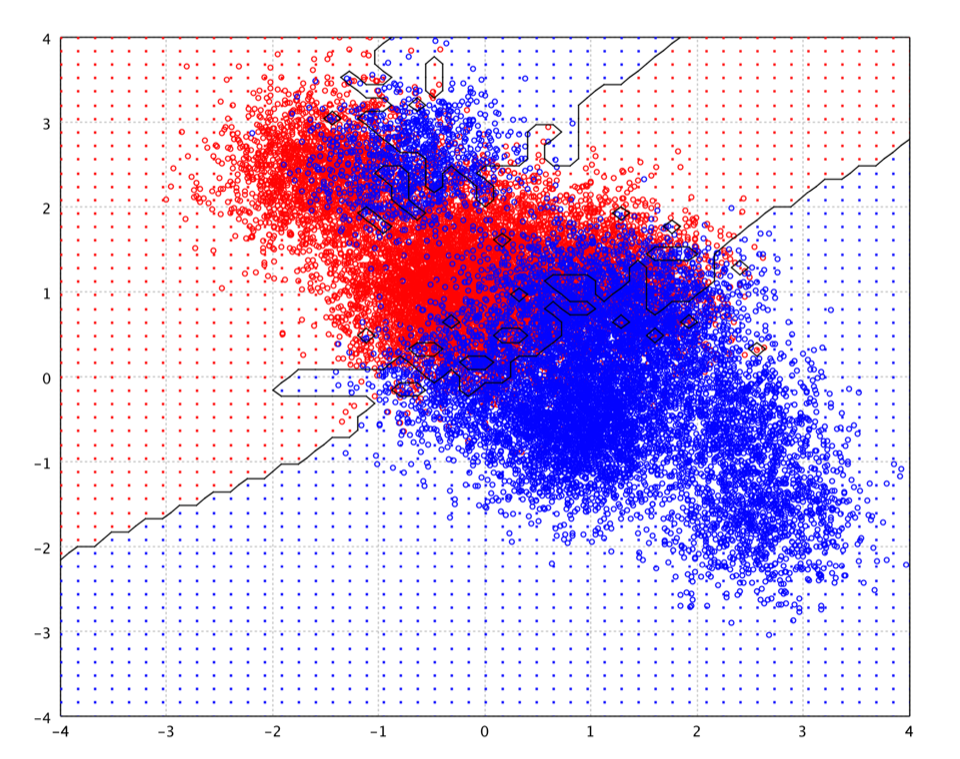
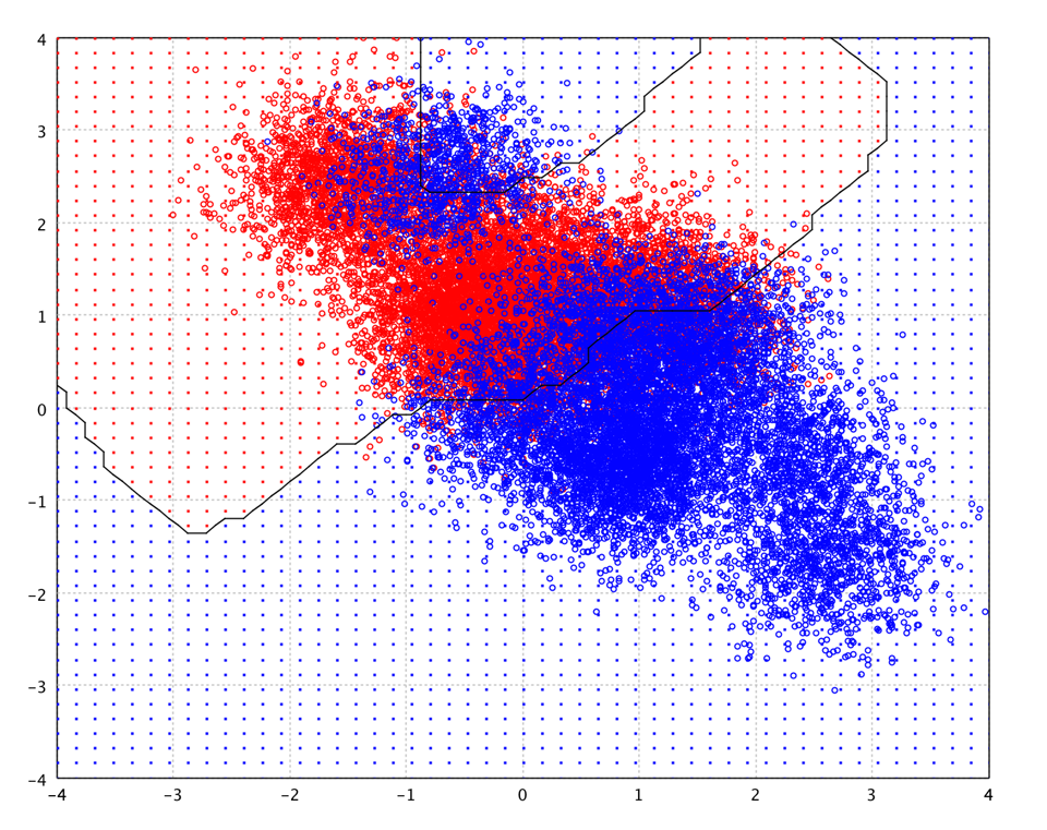
The following picture is the decision boundary of decision tree with 200 nodes on the toy data.

    smile> cart("V1" ~, zip)
    [main] INFO smile.util.package$ - Decision Tree runtime: 0:00:00.754375
    res22: DecisionTree = n=7291
    node), split, n, loss, yval, (yprob)
    * denotes terminal node
    1) root 7291 33095 0 (0.16368 0.13779 0.10026 0.090262 0.089440 0.076291 0.091083 0.088481 0.074373 0.088344)
     2) V214<=-0.999500 3352 12284 1 (0.0077335 0.29655 0.041939 0.028852 0.18233 0.023200 0.012195 0.17995 0.039857 0.18739)
      4) V73<=0.0200000 2109 7264.8 7 (0.0056630 0.017933 0.046720 0.042945 0.26239 0.023124 0.010382 0.26852 0.053799 0.26852)
       8) V25<=-0.862000 578 876.11 4 (0.0034014 0.0017007 0.068027 0.0085034 0.81122 0.018707 0.013605 0.049320 0.018707 0.0068027)
        16) V57<=-0.548000 507 447.15 4 (0.0019342 0.0019342 0.038685 0.0058027 0.89749 0.013540 0.015474 0.0058027 0.013540 0.0058027)
         32) V178<=-0.606000 495 374.13 4 (0.0019802 0.0019802 0.021782 0.0059406 0.91485 0.013861 0.013861 0.0059406 0.013861 0.0059406)
          64) V9<=-0.381000 484 269.82 4 (0.0020243 0.0020243 0.020243 0.0020243 0.93320 0.014170 0.012146 0.0060729 0.0060729 0.0020243)
           128) V146<=0.491500 475 217.48 4 (0.0020619 0.0020619 0.010309 0.0020619 0.94433 0.012371 0.012371 0.0061856 0.0061856 0.0020619)
            256) V207<=0.658500 465 159.07 4 (0.0021053 0.0021053 0.0084211 0.0021053 0.95579 0.0084211 0.0063158 0.0063158 0.0063158 0.0021053) *
            257) V207>0.658500 10 32.941 4 (0.050000 0.050000 0.10000 0.050000 0.25000 0.15000 0.20000 0.050000 0.050000 0.050000)
             514) V90<=-0.996500 5 12.819 4 (0.066667 0.066667 0.13333 0.066667 0.33333 0.066667 0.066667 0.066667 0.066667 0.066667) *
             515) V90>-0.996500 5 14.368 6 (0.066667 0.066667 0.066667 0.066667 0.066667 0.20000 0.26667 0.066667 0.066667 0.066667) *
           129) V146>0.491500 9 25.378 2 (0.052632 0.052632 0.31579 0.052632 0.21053 0.10526 0.052632 0.052632 0.052632 0.052632) *
          65) V9>-0.381000 11 41.156 8 (0.047619 0.047619 0.095238 0.14286 0.095238 0.047619 0.095238 0.047619 0.23810 0.14286)
           130) V71<=-0.979000 6 21.710 3 (0.062500 0.062500 0.12500 0.18750 0.12500 0.062500 0.062500 0.062500 0.062500 0.18750) *
           131) V71>-0.979000 5 12.819 8 (0.066667 0.066667 0.066667 0.066667 0.066667 0.066667 0.13333 0.066667 0.33333 0.066667) *
         33) V178>-0.606000 12 26.958 2 (0.045455 0.045455 0.45455 0.045455 0.13636 0.045455 0.090909 0.045455 0.045455 0.045455) *
        17) V57>-0.548000 71 229.31 7 (0.024691 0.012346 0.25926 0.037037 0.17284 0.061728 0.012346 0.33333 0.061728 0.024691)
         34) V179<=-0.989500 50 139.53 7 (0.016667 0.016667 0.033333 0.033333 0.23333 0.083333 0.016667 0.45000 0.083333 0.033333)
          68) V135<=-0.970000 32 57.888 7 (0.023810 0.023810 0.047619 0.047619 0.047619 0.047619 0.023810 0.64286 0.071429 0.023810)
           136) V183<=-0.987000 26 22.052 7 (0.027778 0.027778 0.027778 0.027778 0.027778 0.055556 0.027778 0.72222 0.027778 0.027778) *
           137) V183>-0.987000 6 23.331 8 (0.062500 0.062500 0.12500 0.12500 0.12500 0.062500 0.062500 0.12500 0.18750 0.062500) *
    ...
    smile> import smile.data.formula.*
    smile> DecisionTree.fit(Formula.lhs("V1"), zip)
    $232 ==> n=7291
    node), split, n, loss, yval, (yprob)
    * denotes terminal node
    1) root 7291 33095 0 (0.16368 0.13779 0.10026 0.090262 0.089440 0.076291 0.091083 0.088481 0.074373 0.088344)
     2) V214<=-0.999500 3352 12284 1 (0.0077335 0.29655 0.041939 0.028852 0.18233 0.023200 0.012195 0.17995 0.039857 0.18739)
      4) V73<=0.0200000 2109 7264.8 7 (0.0056630 0.017933 0.046720 0.042945 0.26239 0.023124 0.010382 0.26852 0.053799 0.26852)
       8) V25<=-0.862000 578 876.11 4 (0.0034014 0.0017007 0.068027 0.0085034 0.81122 0.018707 0.013605 0.049320 0.018707 0.0068027)
        16) V57<=-0.548000 507 447.15 4 (0.0019342 0.0019342 0.038685 0.0058027 0.89749 0.013540 0.015474 0.0058027 0.013540 0.0058027)
         32) V178<=-0.606000 495 374.13 4 (0.0019802 0.0019802 0.021782 0.0059406 0.91485 0.013861 0.013861 0.0059406 0.013861 0.0059406)
          64) V9<=-0.381000 484 269.82 4 (0.0020243 0.0020243 0.020243 0.0020243 0.93320 0.014170 0.012146 0.0060729 0.0060729 0.0020243)
           128) V146<=0.491500 475 217.48 4 (0.0020619 0.0020619 0.010309 0.0020619 0.94433 0.012371 0.012371 0.0061856 0.0061856 0.0020619)
            256) V207<=0.658500 465 159.07 4 (0.0021053 0.0021053 0.0084211 0.0021053 0.95579 0.0084211 0.0063158 0.0063158 0.0063158 0.0021053) *
            257) V207>0.658500 10 32.941 4 (0.050000 0.050000 0.10000 0.050000 0.25000 0.15000 0.20000 0.050000 0.050000 0.050000)
             514) V90<=-0.996500 5 12.819 4 (0.066667 0.066667 0.13333 0.066667 0.33333 0.066667 0.066667 0.066667 0.066667 0.066667) *
             515) V90>-0.996500 5 14.368 6 (0.066667 0.066667 0.066667 0.066667 0.066667 0.20000 0.26667 0.066667 0.066667 0.066667) *
           129) V146>0.491500 9 25.378 2 (0.052632 0.052632 0.31579 0.052632 0.21053 0.10526 0.052632 0.052632 0.052632 0.052632) *
          65) V9>-0.381000 11 41.156 8 (0.047619 0.047619 0.095238 0.14286 0.095238 0.047619 0.095238 0.047619 0.23810 0.14286)
           130) V71<=-0.979000 6 21.710 3 (0.062500 0.062500 0.12500 0.18750 0.12500 0.062500 0.062500 0.062500 0.062500 0.18750) *
           131) V71>-0.979000 5 12.819 8 (0.066667 0.066667 0.066667 0.066667 0.066667 0.066667 0.13333 0.066667 0.33333 0.066667) *
         33) V178>-0.606000 12 26.958 2 (0.045455 0.045455 0.45455 0.045455 0.13636 0.045455 0.090909 0.045455 0.045455 0.045455) *
        17) V57>-0.548000 71 229.31 7 (0.024691 0.012346 0.25926 0.037037 0.17284 0.061728 0.012346 0.33333 0.061728 0.024691)
         34) V179<=-0.989500 50 139.53 7 (0.016667 0.016667 0.033333 0.033333 0.23333 0.083333 0.016667 0.45000 0.083333 0.033333)
          68) V135<=-0.970000 32 57.888 7 (0.023810 0.023810 0.047619 0.047619 0.047619 0.047619 0.023810 0.64286 0.071429 0.023810)
           136) V183<=-0.987000 26 22.052 7 (0.027778 0.027778 0.027778 0.027778 0.027778 0.055556 0.027778 0.72222 0.027778 0.027778) *
           137) V183>-0.987000 6 23.331 8 (0.062500 0.062500 0.12500 0.12500 0.12500 0.062500 0.062500 0.12500 0.18750 0.062500) *
    ...
    >>> import smile.data.formula.*
    >>> cart(Formula.lhs("V1"), zip)
    res160: smile.classification.DecisionTree = n=7291
    node), split, n, loss, yval, (yprob)
    * denotes terminal node
    1) root 7291 33095 0 (0.16368 0.13779 0.10026 0.090262 0.089440 0.076291 0.091083 0.088481 0.074373 0.088344)
     2) V214<=-0.999500 3352 12284 1 (0.0077335 0.29655 0.041939 0.028852 0.18233 0.023200 0.012195 0.17995 0.039857 0.18739)
      4) V73<=0.0200000 2109 7264.8 7 (0.0056630 0.017933 0.046720 0.042945 0.26239 0.023124 0.010382 0.26852 0.053799 0.26852)
       8) V25<=-0.862000 578 876.11 4 (0.0034014 0.0017007 0.068027 0.0085034 0.81122 0.018707 0.013605 0.049320 0.018707 0.0068027)
        16) V57<=-0.548000 507 447.15 4 (0.0019342 0.0019342 0.038685 0.0058027 0.89749 0.013540 0.015474 0.0058027 0.013540 0.0058027)
         32) V178<=-0.606000 495 374.13 4 (0.0019802 0.0019802 0.021782 0.0059406 0.91485 0.013861 0.013861 0.0059406 0.013861 0.0059406)
          64) V9<=-0.381000 484 269.82 4 (0.0020243 0.0020243 0.020243 0.0020243 0.93320 0.014170 0.012146 0.0060729 0.0060729 0.0020243)
           128) V146<=0.491500 475 217.48 4 (0.0020619 0.0020619 0.010309 0.0020619 0.94433 0.012371 0.012371 0.0061856 0.0061856 0.0020619)
            256) V207<=0.658500 465 159.07 4 (0.0021053 0.0021053 0.0084211 0.0021053 0.95579 0.0084211 0.0063158 0.0063158 0.0063158 0.0021053) *
            257) V207>0.658500 10 32.941 4 (0.050000 0.050000 0.10000 0.050000 0.25000 0.15000 0.20000 0.050000 0.050000 0.050000)
             514) V90<=-0.996500 5 12.819 4 (0.066667 0.066667 0.13333 0.066667 0.33333 0.066667 0.066667 0.066667 0.066667 0.066667) *
             515) V90>-0.996500 5 14.368 6 (0.066667 0.066667 0.066667 0.066667 0.066667 0.20000 0.26667 0.066667 0.066667 0.066667) *
           129) V146>0.491500 9 25.378 2 (0.052632 0.052632 0.31579 0.052632 0.21053 0.10526 0.052632 0.052632 0.052632 0.052632) *
          65) V9>-0.381000 11 41.156 8 (0.047619 0.047619 0.095238 0.14286 0.095238 0.047619 0.095238 0.047619 0.23810 0.14286)
           130) V71<=-0.979000 6 21.710 3 (0.062500 0.062500 0.12500 0.18750 0.12500 0.062500 0.062500 0.062500 0.062500 0.18750) *
           131) V71>-0.979000 5 12.819 8 (0.066667 0.066667 0.066667 0.066667 0.066667 0.066667 0.13333 0.066667 0.33333 0.066667) *
         33) V178>-0.606000 12 26.958 2 (0.045455 0.045455 0.45455 0.045455 0.13636 0.045455 0.090909 0.045455 0.045455 0.045455) *
        17) V57>-0.548000 71 229.31 7 (0.024691 0.012346 0.25926 0.037037 0.17284 0.061728 0.012346 0.33333 0.061728 0.024691)
         34) V179<=-0.989500 50 139.53 7 (0.016667 0.016667 0.033333 0.033333 0.23333 0.083333 0.016667 0.45000 0.083333 0.033333)
          68) V135<=-0.970000 32 57.888 7 (0.023810 0.023810 0.047619 0.047619 0.047619 0.047619 0.023810 0.64286 0.071429 0.023810)
           136) V183<=-0.987000 26 22.052 7 (0.027778 0.027778 0.027778 0.027778 0.027778 0.055556 0.027778 0.72222 0.027778 0.027778) *
           137) V183>-0.987000 6 23.331 8 (0.062500 0.062500 0.12500 0.12500 0.12500 0.062500 0.062500 0.12500 0.18750 0.062500) *
    ...
Decision tree techniques have a number of advantages over many of those alternative techniques.
- Simple to understand and interpret:
In most cases, the interpretation of results summarized in a tree is very simple. This simplicity is useful not only for purposes of rapid classification of new observations, but can also often yield a much simpler "model" for explaining why observations are classified or predicted in a particular manner.
- Able to handle both numerical and categorical data:
Other techniques are usually specialized in analyzing datasets that have only one type of variable.
- Nonparametric and nonlinear:
The final results of using tree methods for classification or regression can be summarized in a series of (usually few) logical if-then conditions (tree nodes). Therefore, there is no implicit assumption that the underlying relationships between the predictor variables and the dependent variable are linear, follow some specific non-linear link function, or that they are even monotonic in nature. Thus, tree methods are particularly well suited for data mining tasks, where there is often little a priori knowledge nor any coherent set of theories or predictions regarding which variables are related and how. In those types of data analytics, tree methods can often reveal simple relationships between just a few variables that could have easily gone unnoticed using other analytic techniques.
One major problem with classification and regression trees is their high variance. Often a small change in the data can result in a very different series of splits, making interpretation somewhat precarious. Besides, decision-tree learners can create over-complex trees that cause over-fitting. Mechanisms such as pruning are necessary to avoid this problem. Another limitation of trees is the lack of smoothness of the prediction surface.
Some techniques such as bagging, boosting, and random forest use more than one decision tree for their analysis.
Random Forest
Random forest is an ensemble classifier that consists of many decision trees and outputs the majority vote of individual trees. The method combines bagging idea and the random selection of features.
Each tree is constructed using the following algorithm:
- If the number of cases in the training set is N, randomly sample N cases with replacement from the original data. This sample will be the training set for growing the tree.
- If there are M input variables, a number m << M is specified such that at each node, m variables are selected at random out of the M and the best split on these m is used to split the node. The value of m is held constant during the forest growing.
- Each tree is grown to the largest extent possible. There is no pruning.
    def randomForest(formula: Formula,
                     data: DataFrame,
                     ntrees: Int = 500,
                     mtry: Int = 0,
                     splitRule: SplitRule = SplitRule.GINI,
                     maxDepth: Int = 20,
                     maxNodes: Int = 0,
                     nodeSize: Int = 1,
                     subsample: Double = 1.0,
                     classWeight: Array[Int] = null,
                     seeds: LongStream = null): RandomForest
    public class RandomForest {
        public static RandomForest fit(Formula formula,
                                       DataFrame data,
                                       Options options);
    }
    fun randomForest(formula: Formula,
                     data: DataFrame,
                     ntrees: Int = 500,
                     mtry: Int = 0,
                     splitRule: SplitRule = SplitRule.GINI,
                     maxDepth: Int = 20,
                     maxNodes: Int = 0,
                     nodeSize: Int = 1,
                     subsample: Double = 1.0,
                     classWeight: IntArray = null,
                     seeds: LongStream = null): RandomForest
where ntrees is the number of trees, and mtry is the number
of attributed randomly selected at each node to choose the best split.
Although the original random forest algorithm trains each tree fully without pruning,
it is useful to control the tree size sometimes, which can be achieved by the
parameter maxNodes. The tree can also be regularized by
limiting the minimum number of observations in trees' terminal nodes with the
parameter nodeSize.
When subsample = 1.0, we use the sampling with replacement to train
each tree as described above. If subsample < 1.0, we instead select
a subset of samples (without replacement) to train each tree. If the classes are
not balanced, the user should provide the classWeight (proportional
to the class priori) so that the sampling is done in stratified way. Otherwise,
small classes may be not sampled sufficiently.
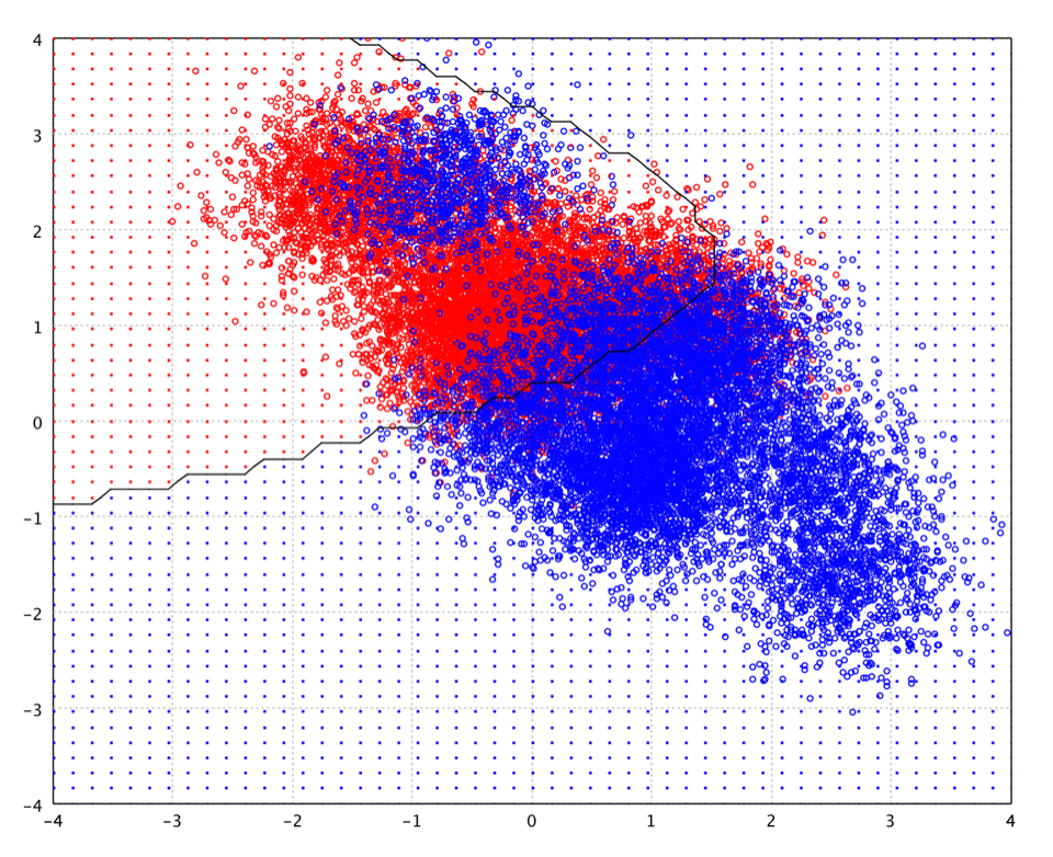
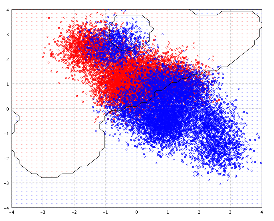
The following picture is the decision boundary of random forest of 100 decision trees with 200 nodes on the toy data.
The advantages of random forest are:
- For many data sets, it produces a highly accurate classifier.
- It runs efficiently on large data sets.
- It can handle thousands of input variables without variable deletion.
- It gives estimates of what variables are important in the classification.
- It generates an internal unbiased estimate of the generalization error as the forest building progresses.
- It has an effective method for estimating missing data and maintains accuracy when a large proportion of the data are missing.
The disadvantages are
- Random forests are prone to over-fitting for some datasets. This is even more pronounced on noisy data.
- For data including categorical variables with different number of levels, random forests are biased in favor of those attributes with more levels. Therefore, the variable importance scores from random forest are not reliable for this type of data.
Gradient Boosted Trees
The idea of gradient boosting originated in the observation that boosting can be interpreted as an optimization algorithm on a suitable cost function. In particular, the boosting algorithms can be abstracted as iterative functional gradient descent algorithms. That is, algorithms that optimize a cost function over function space by iteratively choosing a function (weak hypothesis) that points in the negative gradient direction Gradient boosting is typically used with CART regression trees of a fixed size as base learners.
Generic gradient boosting at the t-th step would fit a regression tree to pseudo-residuals. Let J be the number of its leaves. The tree partitions the input space into J disjoint regions and predicts a constant value in each region. The parameter J controls the maximum allowed level of interaction between variables in the model. With J = 2 (decision stumps), no interaction between variables is allowed. With J = 3 the model may include effects of the interaction between up to two variables, and so on. Hastie et al. comment that typically 4 ≤ J ≤ 8 work well for boosting and results are fairly insensitive to the choice of in this range, J = 2 is insufficient for many applications, and J > 10 is unlikely to be required.
Fitting the training set too closely can lead to degradation of the model's generalization ability. Several so-called regularization techniques reduce this over-fitting effect by constraining the fitting procedure. One natural regularization parameter is the number of gradient boosting iterations T (i.e. the number of trees in the model when the base learner is a decision tree). Increasing T reduces the error on training set, but setting it too high may lead to over-fitting. An optimal value of T is often selected by monitoring prediction error on a separate validation data set.
Another regularization approach is the shrinkage which times a parameter η (called the "learning rate") to update term. Empirically it has been found that using small learning rates (such as η < 0.1) yields dramatic improvements in model's generalization ability over gradient boosting without shrinking (η = 1). However, it comes at the price of increasing computational time both during training and prediction: lower learning rate requires more iterations.
    def gbm(formula: Formula,
            data: DataFrame,
            ntrees: Int = 500,
            maxDepth: Int = 20,
            maxNodes: Int = 6,
            nodeSize: Int = 5,
            shrinkage: Double = 0.05,
            subsample: Double = 0.7): GradientTreeBoost
    public class GradientTreeBoost {
         public static GradientTreeBoost fit(Formula formula,
                                             DataFrame data,
                                             Options options);
    }
    fun gbm(formula: Formula,
            data: DataFrame,
            ntrees: Int = 500,
            maxDepth: Int = 20,
            maxNodes: Int = 6,
            nodeSize: Int = 5,
            shrinkage: Double = 0.05,
            subsample: Double = 0.7): GradientTreeBoost
where ntrees is the number of trees or iterations and shrinkage
is the learning rate.
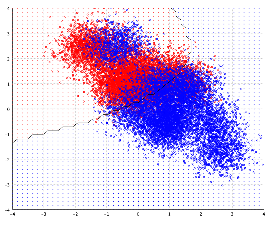
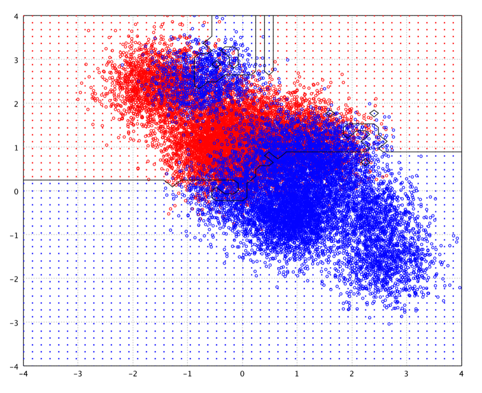
The following picture is the decision boundary of gradient boosted trees of 100 iterations on the toy data.
Soon after the introduction of gradient boosting Friedman proposed a minor modification to the algorithm, motivated by Breiman's bagging method. Specifically, he proposed that at each iteration of the algorithm, a base learner should be fit on a subsample of the training set drawn at random without replacement. Friedman observed a substantial improvement in gradient boosting's accuracy with this modification.
Subsample size is some constant fraction f of the size of the training set. When f = 1, the algorithm is deterministic and identical to the one described above. Smaller values of f introduce randomness into the algorithm and help prevent over-fitting, acting as a kind of regularization. The algorithm also becomes faster, because regression trees have to be fit to smaller datasets at each iteration. Typically, f is set to 0.5, meaning that one half of the training set is used to build each base learner.
Also, like in bagging, sub-sampling allows one to define an out-of-bag estimate of the prediction performance improvement by evaluating predictions on those observations which were not used in the building of the next base learner. Out-of-bag estimates help avoid the need for an independent validation dataset, but often underestimate actual performance improvement and the optimal number of iterations.
AdaBoost
In principle, AdaBoost (Adaptive Boosting) is a meta-algorithm, and can be used in conjunction with many other learning algorithms to improve their performance. In practice, AdaBoost with decision trees is probably the most popular combination. AdaBoost is adaptive in the sense that subsequent classifiers built are tweaked in favor of those instances misclassified by previous classifiers. AdaBoost is sensitive to noisy data and outliers. However, in some problems it can be less susceptible to the over-fitting problem than most learning algorithms.
AdaBoost calls a weak classifier repeatedly in a series of rounds from total T classifiers. For each call a distribution of weights is updated that indicates the importance of examples in the data set for the classification. On each round, the weights of each incorrectly classified example are increased (or alternatively, the weights of each correctly classified example are decreased), so that the new classifier focuses more on those examples.
    def adaboost(formula: Formula,
                 data: DataFrame,
                 ntrees: Int = 500,
                 maxDepth: Int = 20,
                 maxNodes: Int = 6,
                 nodeSize: Int = 1): AdaBoost
    public class AdaBoost {
         public static AdaBoost fit(Formula formula,
                                    DataFrame data,
                                    Options options);
    }
    fun adaboost(formula: Formula,
                 data: DataFrame,
                 ntrees: Int = 500,
                 maxDepth: Int = 20,
                 maxNodes: Int = 6,
                 nodeSize: Int = 1): AdaBoost
The following picture is the decision boundary of AdaBoost of 100 trees on the toy data.

The basic AdaBoost algorithm is only for binary classification problem. For multi-class classification, a common approach is reducing the multi-class classification problem to multiple two-class problems. SMILE implements a multi-class AdaBoost without such reductions.